
Yang-Zhang Volatility in Python
How to Code Yang-Zhang Volatility For Time Series Analysis


The Yang-Zhang volatility estimator is a measure of historical volatility that combines the advantages of both the Rogers-Satchell and Garman-Klass estimators. It is particularly useful for assets with high opening jumps or overnight gaps. This estimator is designed to reduce the bias and error present in simpler volatility estimators.
This article presents this volatility measure in detail and shows how to code a rolling calculation on time series using Python.
Understanding Yang-Zhang Volatility
Before discussing complex volatility models, it is always recommended to have a thorough understanding of the most basic volatility model (or calculation), that is the historical standard deviation. The standard deviation using the historical method is a common way to measure the volatility of a financial instrument based on past price data.
It quantifies the amount of variation or dispersion of a set of values. In finance, it typically measures the dispersion of daily returns around their mean. Follow these steps to calculate the standard deviation:
Calculate the returns using either the differencing (first function) or the log method (second function).


Calculate the average (mean) of the returns:

Compute the variance of the daily returns:

The standard deviation is the square root of the variance:

Like any statistical measure, it has its advantages and disadvantages. The historical standard deviation is straightforward to compute. It requires basic statistical operations that can be easily implemented in spreadsheets and programming languages. It is a well-understood measure of variability and is easy to explain to stakeholders who may not have a deep statistical background. Many financial models and risk metrics (such as the Sharpe ratio) rely on standard deviation as a measure of risk.
For small sample sizes, the historical standard deviation tends to underestimate true volatility. This bias can lead to misleading conclusions about the risk of an asset. The method assumes that the underlying volatility of the asset is constant over the period being analyzed. In reality, volatility can change over time, making this assumption unrealistic.
Additionally, financial returns often exhibit fat tails (leptokurtosis) and skewness, meaning they do not follow a normal distribution. The standard deviation does not capture these characteristics, potentially underestimating risk.
Use the following code in Python to calculate a rolling 5-day measure of volatility on Nvidia’s daily returns:
import numpy as np
import matplotlib.pyplot as plt
import yfinance as yf

def calculate_rolling_historical_volatility(data, window):
    # Calculate returns (using the differencing method)
    returns = data['Close'] - data['Close'].shift(1).dropna()

    # Calculate the rolling standard deviation of the returns
    rolling_volatility = returns.rolling(window=window).std()

    # return a variable containing standard deviation measures
    return rolling_volatility

# download the historical values of Nvidia
df = yf.download("NVDA", start = "2022-01-01", end = "2024-06-30")

# Define the rolling window size
window_size = 5

# apply the formula and get the volatility data frame
rolling_volatility = calculate_rolling_historical_volatility(df, window=window_size)

# plot volatility across time
plt.plot(rolling_volatility, color = 'black', label = '5-period historical standard deviation')
plt.legend()
plt.grid()
plt.axhline(y = np.mean(rolling_volatility), color = 'red', linestyle = 'dashed')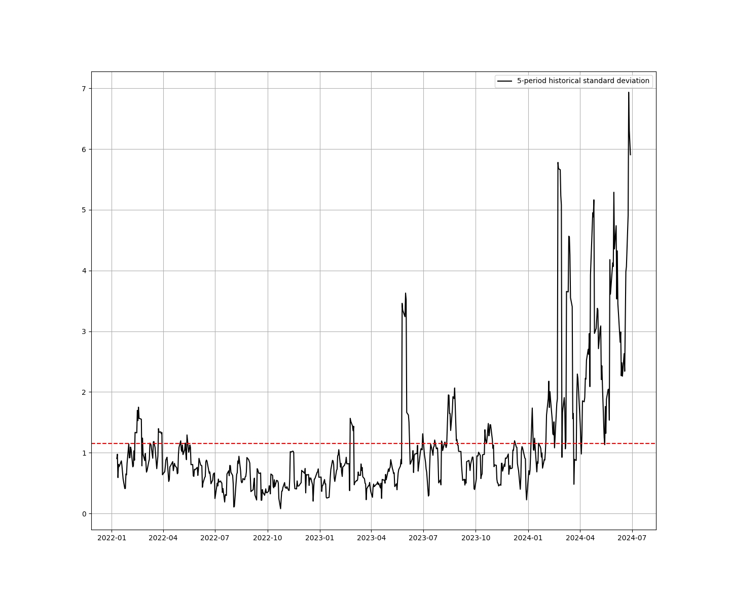
The Yang-Zhang volatility estimator is a measure of historical volatility that combines the advantages of both the Rogers-Satchell and Garman-Klass estimators. It is particularly useful for assets with high opening jumps or overnight gaps. This estimator is designed to reduce the bias and error present in simpler volatility estimators.
The Yang-Zhang volatility estimator is calculated using the following formula:

With:

And the first standard deviation term refers to the open-close volatility, the second to the close-close volatility, and the third is the Rogers-Satchell volatility estimator.
The K factor balances the contribution of open-close volatility and close-close volatility, adjusting for sample size n. The Yang-Zhang estimator is less sensitive to opening price jumps and closing price variations compared to other estimators, making it more robust for assets that experience significant overnight gaps.
Do you want to master Deep Learning techniques tailored for time series, trading, and market analysis🔥? My book breaks it all down from basic machine learning to complex multi-period LSTM forecasting while going through concepts such as fractional differentiation and forecasting thresholds. Get your copy here 📖!
Calculating Yang-Zhang Volatility in Python
Let’s now use Python to calculate Yang-Zhang volatility. We will use the same example (i.e. Nvidia’s daily returns with a lookback period of 5):
import numpy as np
import matplotlib.pyplot as plt
import yfinance as yf
import math

def yang_zhang(price_data, window_size = 30, periods = 252, clean = True):

    log_ho = (price_data["High"] / price_data["Open"]).apply(np.log)
    log_lo = (price_data["Low"] / price_data["Open"]).apply(np.log)
    log_co = (price_data["Close"] / price_data["Open"]).apply(np.log)

    log_oc = (price_data["Open"] / price_data["Close"].shift(1)).apply(np.log)
    log_oc_sq = log_oc ** 2

    log_cc = (price_data["Close"] / price_data["Close"].shift(1)).apply(np.log)
    log_cc_sq = log_cc ** 2

    rs = log_ho * (log_ho - log_co) + log_lo * (log_lo - log_co)

    close_vol = log_cc_sq.rolling(window=window_size, center=False).sum() * (
        1.0 / (window_size - 1.0)
    )
    open_vol = log_oc_sq.rolling(window=window_size, center=False).sum() * (
        1.0 / (window_size - 1.0)
    )
    window_rs = rs.rolling(window=window_size, center=False).sum() * (1.0 / (window_size - 1.0))

    k = 0.34 / (1.34 + (window_size + 1) / (window_size - 1))
    result = (open_vol + k * close_vol + (1 - k) * window_rs).apply(
        np.sqrt
    ) * math.sqrt(periods)

    if clean:
        return result.dropna()
    else:
        return result


# download the historical values of Nvidia
df = yf.download("NVDA", start = "2020-01-01", end = "2024-06-30")
# Define the rolling window size
window_size = 5
# apply the formula and get the volatility data frame
rolling_volatility = yang_zhang(df)
# plot volatility across time
plt.plot(rolling_volatility, color = 'black', label = '5-period Yang-Zhang volatility')
plt.legend()
plt.grid()
plt.axhline(y = np.mean(rolling_volatility), color = 'red', linestyle = 'dashed')
The code is inspired from pyquant.news.

The historical standard deviation is a useful and widely adopted measure of volatility due to its simplicity, ease of calculation, and general acceptance in the financial industry. However, its limitations, particularly in handling small sample sizes, non-stationary volatility, and the non-normal distribution of returns, suggest that it should be used with caution.
In situations where accuracy is paramount or sample sizes are small, alternative volatility models may provide better risk assessments.
Every week, I analyze positioning, sentiment, and market structure. Curious what hedge funds, retail, and smart money are doing each week? Then join hundreds of readers here in the Weekly Market Sentiment Report 📜 and stay ahead of the game through chart forecasts, sentiment analysis, volatility diagnosis, and seasonality charts.
Free trial available🆓
