


Kernel Ridge Regression (KRR), sits at an interesting point between classical linear models and modern kernel methods. It keeps the structure of Ridge Regression but uses kernels to model nonlinear patterns.
This lets it handle complex relationships with a relatively simple mathematical foundation.
Introduction
Regression methods often end up caught between underfitting and overfitting. Linear models lose power when relationships curve or twist in ways a straight line cannot capture.
More flexible models can overreact to noise. KRR offers a balanced alternative. It combines the stability of Ridge Regression with the flexibility of kernel functions, which expand the input space without explicitly computing higher dimensional features. The result is a model that can adapt to nonlinear data while keeping training stable.
Ridge Regression minimizes a squared error loss with a penalty on the magnitude of model weights. Formally, for data matrix X and target vector y, Ridge solves:

The regularization term λ∥w∥ controls model complexity. Larger λ shrinks the weights and reduces the risk of overfitting.
Linear Ridge Regression can be rewritten in a dual form that depends only on inner products between samples. Replace those inner products with a kernel function k(xi,xj) and the model can learn nonlinear boundaries. Popular kernels include:
Gaussian (RBF) kernel
Polynomial kernel
Sigmoid kernel
Linear kernel (as a baseline)
These functions measure similarity between data points in ways that emulate high dimensional feature mappings. KRR solves the system:

where K is the kernel matrix. Predictions for a new input x follow:

This solution is simple, but computing K and inverting K+λI are both expensive when the dataset is large.
🚨 Get your Quant Atlas Free trial (no credit card required) 🚨
Sign up takes ~9 seconds before you have unconditional 10-day access to 100+ market forecasts.
Understanding the Hyperparameters
Regularization strength (λ)
Controls the bias-variance tradeoff. Smaller values allow the model to fit the training data more tightly. Larger values promote smoother functions.
Kernel choice
The kernel defines the geometry of the model’s hypothesis space. An RBF kernel gives smooth, flexible functions. A polynomial kernel introduces interactions of controlled degree. Kernel choice shapes what patterns the model can learn.
Kernel parameters
For example, the RBF kernel uses a bandwidth parameter γ. A small γ creates a broad influence for each data point. A large γ makes the model sensitive to small variations.
Implementing the KRR
Suppose we have a sine wave-like time series like the following and we want to predict the rest of the sequence.
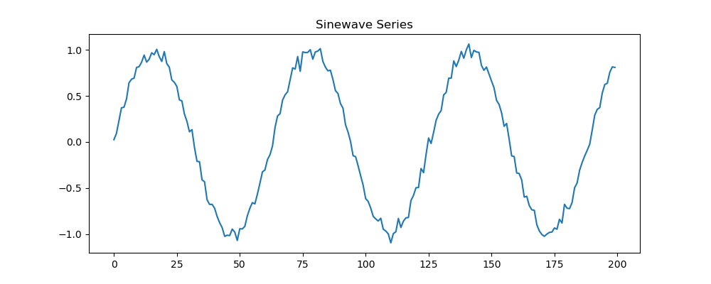
We will use the algorithm to implement the experiment:
import numpy as np
import matplotlib.pyplot as plt
from sklearn.kernel_ridge import KernelRidge
from sklearn.preprocessing import StandardScaler

np.random.seed(42)

n = 1000
x = np.arange(n)
y = np.sin(0.1 * x)  + np.random.normal(0, 0.05, size=n)

plt.figure(figsize=(10, 4))
plt.plot(x, y)
plt.title(”Sinewave Series”)
plt.show()

def make_lag_features(y, nlags=5):
    data = {}
    for i in range(1, nlags + 1):
        data[f”lag{i}”] = np.roll(y, i)
    df = np.column_stack([data[f”lag{i}”] for i in range(1, nlags + 1)])
    # Fix first rows
    for i in range(nlags):
        df[i, :] = y[0]
    return df

nlags = 50
X = make_lag_features(y, nlags)

# Scale the lag matrix
scaler = StandardScaler()
X_scaled = scaler.fit_transform(X)

model = KernelRidge(kernel=”rbf”, alpha=0.1, gamma=1.0)
model.fit(X_scaled, y)

future_steps = 50
forecast = []

# Start from the last observed segment of lags
history = list(y.copy())

for step in range(future_steps):
    # Build lag vector from latest values
    lags = [history[-i] for i in range(1, nlags + 1)]
    row = np.array(lags).reshape(1, -1)

    # Scale features
    row_scaled = scaler.transform(row)

    # Predict next value
    next_val = model.predict(row_scaled)[0]

    # Store prediction
    forecast.append(next_val)

    # Add it to history so next step uses it as a lag
    history.append(next_val)

future_x = np.arange(n, n + future_steps)

plt.figure(figsize=(12, 4))
plt.plot(x, y, label=”Training series”)
plt.plot(future_x, forecast, label=”Recursive forecast”)
plt.legend()
plt.title(”Recursive Kernel Ridge Forecast with Lag Features”)
plt.show()
The following is the output of the code.
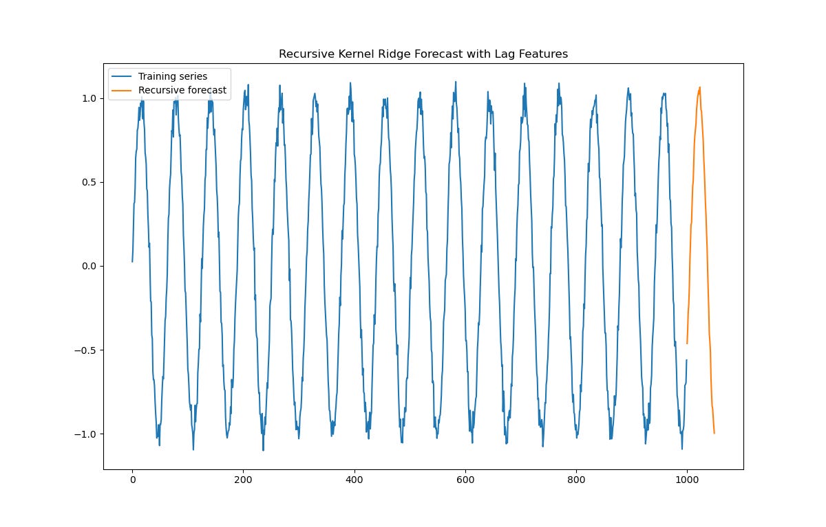
Notice how the algorithm succeeds at capturing the oscillating nature of the time series.
KRR offers a clean and stable way to build nonlinear models. It unites the strengths of regularization and kernel methods in a simple mathematical framework.