Wavelet Transform Modulus Maxima For Time Series Analysis
Transform this Powerful Technique to a Technical Indicator


This is one of the most elegant techniques in multifractal analysis and nonlinear time series, and it sits at the heart of using wavelets for detecting singularities (sharp transitions) in complex systems like financial markets.
Let’s understand this technique and apply it in market analysis.
Introduction to Wavelet Transform Modulus Maxima
The Wavelet Transform Modulus Maxima (WTMM) method is an analytical framework for studying the fractal and multifractal properties of nonstationary signals.
It was introduced by Arneodo, Bacry, and Muzy (1995) as a robust alternative to classical box-counting or DFA methods.
Where traditional Fourier transforms give global frequency content, the Continuous Wavelet Transform (CWT) gives you scale–time localization.
The WTMM method then extracts the geometric skeleton of the signal, the set of sharp local variations that define its structure across scales.
Given a signal x(t), the CWT is defined as:
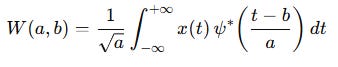
where:
a = scale parameter (zoom level)
b = translation parameter (position in time)
ψ(t) = mother wavelet (a short oscillating function)
* denotes complex conjugation
This transform maps a 1D time series x(t) into a 2D surface W(a,b) showing how local patterns evolve with scale. The modulus of the wavelet coefficient is:
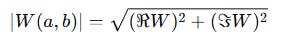
The WTMM method identifies points where ∣W(a,b)∣ is locally maximal in time b for each scale a.
These are called the modulus maxima lines (or ridges).
Intuitively:
A ridge represents a local singularity: a sharp slope change, like a turning point or volatility burst.
As you go across scales, these ridges form chains: showing how singularities propagate through time and scale.
The full set of ridges forms the WTMM skeleton of the signal.
WTMM provides a multi-scale map of singularities. Each ridge corresponds to a local irregularity or trend transition. By following these ridges across scales, you can analyze the hierarchical (fractal) structure of a signal.
Mathematically, you can estimate the Lipschitz (Hölder) exponent α(t) of each singularity from how the wavelet modulus decays with scale:
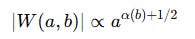
This α(b) is the local regularity exponent:
Large α → smooth region (trend)
Small α → irregular region (shock, reversal)
Plotting the spectrum of α values gives the multifractal spectrum, a fingerprint of structural complexity. We’ll call this indicator we’re going to create: The Fractal Signal Index
I started Quant Atlas, a platform for Quantitative forecasting through charts, powered by multiple models working together. 📈
No noise. No guesswork. Just structured, data-driven market forecasts across assets.
If you want to see how it actually performs in real time, you can try it yourself.
Creating the Fractal Strength Index
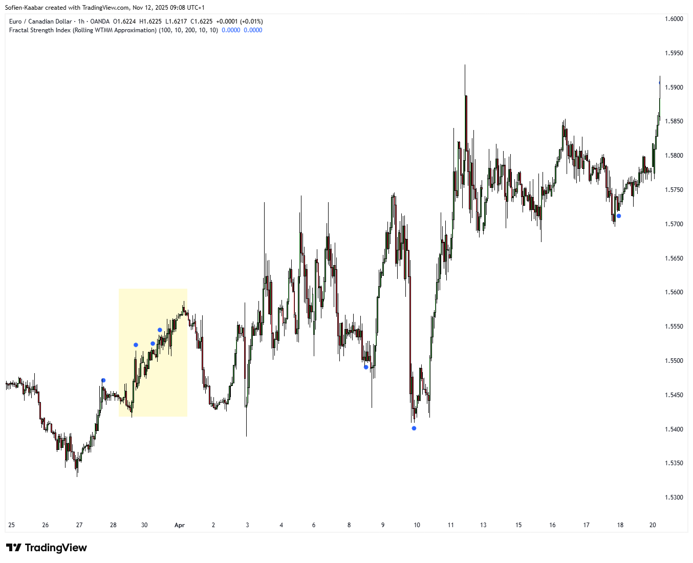
Let’s now create the Fractal Strength Index (FSI) in Pine Script so that we can visualize it alongside the market price and detect local tops and bottoms.
The FSI is overlay and will show as:
A blue dot below the market price when a bullish reversal is expected.
A blue dot above the market price when a bearish reversal is expected.
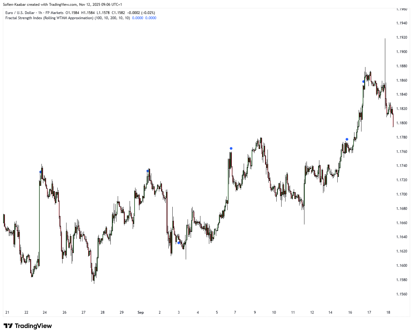
Typically, it comes around the end of a local/intermediate trend. Despite it being not perfect, it manages to capture the chaotic nature of financial time series quite well.
It can also be used as a tool to follow the trend.
Blue dots below the market appearing in a bullish trend can signal a good bullish opportunity.
Blue dots above the market appearing in a bearish trend can signal a good bearish opportunity.
Use the following code to implement the FSI:
//@version=5
indicator(”Fractal Strength Index (Rolling WTMM Approximation)”, overlay=true, max_bars_back=500)

len      = input.int(256, “Rolling window”, minval=32)
minScale = input.int(10, “Minimum scale”, minval=2)
maxScale = input.int(100, “Maximum scale”, minval=8)
scaleStep = input.int(2, “Scale step”, minval=1)
smoothLen = input.int(5, “Smoothing (EMA)”, minval=1)

normClose = (close - ta.sma(close, len)) / ta.stdev(close, len)

// We use Gaussian-like filters as causal approximations of wavelet energy
var float strength = na
sumEnergy = 0.0
count = 0.0

for scale = minScale to maxScale by scaleStep
    // rolling difference approximates local curvature at each scale
    up   = normClose - ta.sma(normClose, scale)
    energy = math.abs(up)
    sumEnergy += energy
    count += 1

fsi_raw = sumEnergy / count
fsi = ta.ema(fsi_raw, smoothLen)

// Normalize between 0–1 dynamically
fsi_min = ta.lowest(fsi, len)
fsi_max = ta.highest(fsi, len)
fsi_norm = (fsi - fsi_min) / math.max(fsi_max - fsi_min, 1e-6)

plotshape(fsi_norm == 1 and fsi_norm[1] == 1 and fsi_norm[2] < 1 and ta.rsi(close, 8) < 40,  style = shape.circle, color = color.blue, location =  location.belowbar, size = size.tiny)
plotshape(fsi_norm == 1 and fsi_norm[1] == 1 and fsi_norm[2] < 1 and  ta.rsi(close, 8) > 60,  style = shape.circle, color = color.blue, location =  location.abovebar, size = size.tiny)
It’s important to know the limitations of indicators as they only use past data. Sometimes, the trend is too strong and sometimes the indicator fails to capture the on-going nature of the market.