
Using Technical Indicators to Determine the Market’s Regime.
A Visual Way of Using Technical Indicators to Understand the Current Regime.


Color-coding charts can be helpful to determine the market’s state when we want to take a quick glance at the charts. True we might be able to determine the trend visually or by using moving averages, but we can also use other indicators and transform the chart so that it reflects the indicator’s values. This article will discuss how to do that. The aim is to be able to produce multiple charts at the same time with a color code that shows our conditions.
I have just published a new book after the success of my previous one “New Technical Indicators in Python”. It features a more complete description and addition of structured trading strategies with a Github page dedicated to the continuously updated code. If you feel that this interests you, feel free to visit the below link, or if you prefer to buy the PDF version, you could contact me on Linkedin.
The Book of Trading Strategies
Amazon.com: The Book of Trading Strategies: 9798532885707: Kaabar, Sofien: Bookswww.amazon.com
Fetching Historical OHLC Data
One of the most famous trading platforms in the retail community is the MetaTrader5 software. It is a powerful tool that comes with its own programming language and its huge online community support. It also offers the possibility to export its historical short-term and long-term FX data.
The first thing we need to do is to simply download the platform from the official website. Then, after creating the demo account, we are ready to import the library in Python that allows to import the OHLC data from MetaTrader5.
A library is a group of structured functions that can be imported into our Python interpreter from where we can call and use the ones we want.
The easiest way to install the MetaTrader5 library is to go to the Python prompt on our computer and type:
pip install MetaTrader5This should install the library in our local Python. Now, we want to import it to the Python interpreter (such as Pycharm or SPYDER) so that we can use it. Let us actually import all the libraries we will be using for this:
import datetime                 # Date acquiring
import pytz                     # Time zone management
import pandas            as pd  # Mostly for Data frame manipulation
import MetaTrader5       as mt5 # Importing OHLC data
import matplotlib.pyplot as plt # Plotting charts
import numpy             as np  # Mostly for array manipulation
Anything that comes after “as” is a shortcut. The plt shortcut is there so that each time we want to call a function from that library we do not have to type the full matplotlib.pyplot statement.
The official documentation for the Metatrader5 libary can be found here.
The first thing we can do is to select which time frame we want to import. Let us suppose that there are only two time frames, the 30-minute and the hourly bars. We can therefore create variables that hold the statement to tell the MetaTrader5 library which time frame we want.
# Choosing the 30-minute time frame
frame_M30  = mt5.TIMEFRAME_M30

# Choosing the hourly time frame
frame_H1   = mt5.TIMEFRAME_H1
Then, by staying in the spirit of importing variables, we can define the variable that states what date is it now. This helps the algorithm know the stopping date of the import. We can do this by the simple line of code below.
# Defining the variable now to give out the current date
now = datetime.datetime.now()
Note that these code snippets are better used chronologically, hence, I encourage you to copy them in order and then execute them one by one so that you understand the evolution of what you are doing. The below is a function that holds which assets we want. Generally, I use 10 or more but for simplicity, let us consider that there are only two currency pairs: EURUSD and USDCHF.
def asset_list(asset_set):

    if asset_set == 'FX':assets = ['EURUSD', 'USDCHF']
return assetsNow, with the key function that gets us the OHLC data. The below establishes a connection to MetaTrader5, applies the current date, and extracts the needed data. Notice the arguments year, month, and day. These will be filled by us to select from when do we want the data to start. Note, I have inputed Europe/Paris as my time zone, you should use your time zone to get more accurate data.
def get_quotes(time_frame, year = 2005, month = 1, day = 1, asset = "EURUSD"):

    # Establish connection to MetaTrader 5
    if not mt5.initialize():
        print("initialize() failed, error code =", mt5.last_error())
        quit()

    timezone = pytz.timezone("Europe/Paris")

    utc_from = datetime.datetime(year, month, day, tzinfo = timezone)
    utc_to = datetime.datetime(now.year, now.month, now.day + 1, tzinfo = timezone)

    rates = mt5.copy_rates_range(asset, time_frame, utc_from, utc_to)

    rates_frame = pd.DataFrame(rates)
return rates_frameAnd finally, the last function we will use is the one that uses the below get_quotes function and then cleans the results so that we have a nice array. We have selected data since January 2019 as shown below.
def mass_import(asset, horizon):

 if horizon == 'M30':
   data = get_quotes(frame_M30, 2019, 1, 1, asset = assets[asset])
   data = data.iloc[:, 1:5].values
   data = data.round(decimals = 5)return data
Finally, we are done building the blocks necessary to import the data. To import EURUSD OHLC historical data, we simply use the below code line:
# Choosing the horizon
horizon = 'M30'
# Creating an array called EURUSD having M30 data since 2019
EURUSD = mass_import(0, horizon)And voila, now we have the EURUSD OHLC data from 2019.
The Market’s Regime
The market regime is its current state and can be divided into:
Bullish trend: The market has a tendency to make higher highs meaning that the aggregate direction is upwards.
Sideways: The market has a tendency to to range while remaining within established zones.
Bearish trend: The market has a tendency to make lower lows meaning that the aggregate direction is downwards.
Many tools attempt to detect the trend and most of them do give the answer but we can not really say we can predict the next state. The best way to solve this issue is to assume that the current state will continue and trade any reactions, preferably in the direction of the trend. For example, if the EURUSD is above its moving average and shaping higher highs, then it makes sense to wait for dips before buying and assuming that the bullish state will continue, also known as a trend-following strategy.

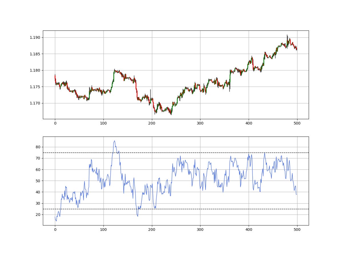
The above chart shows the EURUSD’s hourly values where the market trended upwards for a while before reversing. Now, we will discuss a simple technical indicator called the RSI and see how we can color code the trend for more objectivity.
The Relative Strength Index
The RSI is without a doubt the most famous momentum indicator out there, and this is to be expected as it has many strengths especially in ranging markets. It is also bounded between 0 and 100 which makes it easier to interpret. Also, the fact that it is famous, contributes to its potential.
This is because the more traders and portfolio managers look at the RSI, the more people will react based on its signals and this in turn can push market prices. Of course, we cannot prove this idea, but it is intuitive as one of the basis of Technical Analysis is that it is self-fulfilling.
The RSI is calculated using a rather simple way. We first start by taking price differences of one period. This means that we have to subtract every closing price from the one before it. Then, we will calculate the smoothed average of the positive differences and divide it by the smoothed average of the negative differences. The last calculation gives us the Relative Strength which is then used in the RSI formula to be transformed into a measure between 0 and 100.
To calculate the Relative Strength Index, we need an OHLC array (not a data frame). This means that we will be looking at an array of 4 columns. The function for the Relative Strength Index is therefore:
def adder(Data, times):

    for i in range(1, times + 1):

        new = np.zeros((len(Data), 1), dtype = float)
        Data = np.append(Data, new, axis = 1)

    return Data
def deleter(Data, index, times):
for i in range(1, times + 1):
Data = np.delete(Data, index, axis = 1)
return Data
def jump(Data, jump):
Data = Data[jump:, ]
return Datadef ma(Data, lookback, close, where):
Data = adder(Data, 1)
for i in range(len(Data)):
try:
Data[i, where] = (Data[i - lookback + 1:i + 1, close].mean())
except IndexError:
pass
# Cleaning
Data = jump(Data, lookback)
return Datadef ema(Data, alpha, lookback, what, where):
alpha = alpha / (lookback + 1.0)
beta = 1 - alpha
# First value is a simple SMA
Data = ma(Data, lookback, what, where)
# Calculating first EMA
Data[lookback + 1, where] = (Data[lookback + 1, what] * alpha) + (Data[lookback, where] * beta)
# Calculating the rest of EMA
for i in range(lookback + 2, len(Data)):
try:
Data[i, where] = (Data[i, what] * alpha) + (Data[i - 1, where] * beta)
except IndexError:
pass
return Datadef rsi(Data, lookback, close, where, width = 1, genre = 'Smoothed'):
# Adding a few columns
Data = adder(Data, 7)
# Calculating Differences
for i in range(len(Data)):
Data[i, where] = Data[i, close] - Data[i - width, close]
# Calculating the Up and Down absolute values
for i in range(len(Data)):
if Data[i, where] > 0:
Data[i, where + 1] = Data[i, where]
elif Data[i, where] < 0:
Data[i, where + 2] = abs(Data[i, where])
# Calculating the Smoothed Moving Average on Up and Down
absolute values
if genre == 'Smoothed':
lookback = (lookback * 2) - 1 # From exponential to smoothed
Data = ema(Data, 2, lookback, where + 1, where + 3)
Data = ema(Data, 2, lookback, where + 2, where + 4)
if genre == 'Simple':
Data = ma(Data, lookback, where + 1, where + 3)
Data = ma(Data, lookback, where + 2, where + 4)
# Calculating the Relative Strength
Data[:, where + 5] = Data[:, where + 3] / Data[:, where + 4]
# Calculate the Relative Strength Index
Data[:, where + 6] = (100 - (100 / (1 + Data[:, where + 5])))
# Cleaning
Data = deleter(Data, where, 6)
Data = jump(Data, lookback) return Data
The Relative Strength Index is known for the extremes strategy (Oversold and Overbought levels) where we initiate contrarian positions when the RSI is close to the extremes in an attempt to fade the current trend.
Creating the Visual Interpreter
The assumption we will be making is that the RSI is a momentum indicator where values above 50 signify a bullish net momentum and values below 50 signify a bearish net momentum.
We will calculate a 55-period RSI on the market price and then color code the bar charts in green if the RSI above 50 and we will color code them in red if the RSI is below 50.
lookback = 55
my_data  = rsi(my_data, lookback, 3, 4)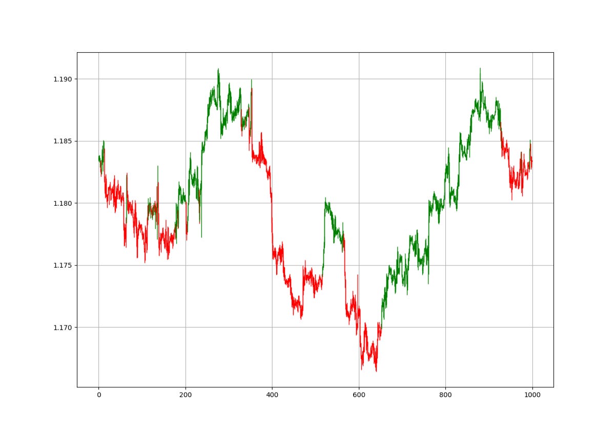
The code to generate the above chart lies with this function below.
def ohlc_plot_candles(Data, window):

    Chosen = Data[-window:, ]

    for i in range(len(Chosen)):

        if Chosen[i, 4] > 50:
            plt.vlines(x = i, ymin = Chosen[i, 2], ymax = Chosen[i, 1], color = 'green', linewidth = 1)
            color_chosen = 'green'
            plt.vlines(x = i, ymin = Chosen[i, 0], ymax = Chosen[i, 3], color = color_chosen, linewidth = 1)
if Chosen[i, 4] < 50:
plt.vlines(x = i, ymin = Chosen[i, 2], ymax = Chosen[i, 1], color = 'red', linewidth = 1)
color_chosen = 'red'
plt.vlines(x = i, ymin = Chosen[i, 3], ymax = Chosen[i, 0], color = color_chosen, linewidth = 1)
plt.grid()You have to make sure you have the OHLC array imported the right way with an RSI next to it.

When we see a cluster of green values, we know that it is a bullish state as the 55-period RSI is telling us that the momentum is positive. Of course, there can be false signals in sideway moving markets such as the USDCHF evidenced in the chart above.

The above example shows the AUDCAD with the colors that clearly indicate the current regime. This is but a simple way to understand the regime. Now, let us try changing the lookback of the RSI to 144 and apply it on the same AUDCAD chart.
lookback = 144
As expected, there are less false signals but more lag. The method is a trade-off between confirmation and wanting to get in early. My recommendation is to combine this technique with classical charting methods such as trend lines. Let us see an example on the same AUDCAD chart to understand what I am saying.

Notice the surpassed trend line that has been acting as resistance. Now, we can see the confirmation from the chart turning green. This is referred to as a bullish confirmation strategy.
If you are also interested by more technical indicators and using Python to create strategies, then my best-selling book on Technical Indicators may interest you:
New Technical Indicators in Python
Amazon.com: New Technical Indicators in Python: 9798711128861: Kaabar, Mr Sofien: Bookswww.amazon.com
Conclusion
Remember to always do your back-tests. You should always believe that other people are wrong. My indicators and style of trading may work for me but maybe not for you.
I am a firm believer of not spoon-feeding. I have learnt by doing and not by copying. You should get the idea, the function, the intuition, the conditions of the strategy, and then elaborate (an even better) one yourself so that you back-test and improve it before deciding to take it live or to eliminate it. My choice of not providing specific Back-testing results should lead the reader to explore more herself the strategy and work on it more.
To sum up, are the strategies I provide realistic? Yes, but only by optimizing the environment (robust algorithm, low costs, honest broker, proper risk management, and order management). Are the strategies provided only for the sole use of trading? No, it is to stimulate brainstorming and getting more trading ideas as we are all sick of hearing about an oversold RSI as a reason to go short or a resistance being surpassed as a reason to go long. I am trying to introduce a new field called Objective Technical Analysis where we use hard data to judge our techniques rather than rely on outdated classical methods.