Using LSTM to Predict Stock Volatility Using Data From FMP
Creating a Volatility Auto-Regressive Forecast Model Using LSTM
Neural networks, including their specialized forms like LSTMs, have revolutionized machine learning and artificial intelligence. By mimicking the brain’s structure and learning from data, they enable machines to perform tasks that were once thought to be exclusively human domains.
Understanding the basics of neural networks and the unique advantages of LSTMs provides a solid foundation for exploring more advanced topics and applications in the field.
This article will introduce these complex structures and show how to predict the volatility of Apple’s stock price using data imported from FMP.
A Primer in Neural Networks and LSTMs
Neural networks are a class of machine learning algorithms inspired by the human brain’s structure and function. They consist of interconnected nodes or neurons that work together to solve complex problems. Neural networks are particularly well-suited for tasks involving pattern recognition, classification, regression, and generation of new data. The basic structure of a neural network is composed of mainly three elements:
Input layer: The first layer, where the network receives input data. This is the equivalent of your independent variables (the predictors)
Hidden layer(s): Intermediate layers that process inputs received from the input layer. There can be multiple hidden layers in a network. This is the equivalent of the weighting and math done during the training.
Output layer: The final layer, which produces the output of the network. This is the equivalent of the forecast (prediction) of the model.
Each neuron in a layer is connected to neurons in the previous and next layers. These connections have associated weights, which are adjusted during training to minimize the error in predictions.
But how does the process work? First, there is the forward propagation where data is fed into the input layer, then processed through the hidden layers via weighted connections and activation functions (e.g., sigmoid, tanh, ReLU). Finally, the processed data reaches the output layer, producing a prediction.
Within all this, the backpropagation is being processed; the error between the predicted output and the actual output is calculated using a loss function (e.g., mean squared error, cross-entropy). The error is propagated back through the network. Weights are adjusted using optimization algorithms (e.g., gradient descent) to minimize the error.
There are many types of neural networks. The one discussed above is the simples and is called a feedforward neural network. This is where connections between nodes do not form cycles. Data moves in one direction, from input to output. A more advanced type is referred to as recurrent neural networks (RNNs). Designed for sequential data, they maintain a memory of previous inputs, making them suitable for tasks like time series prediction and language modeling.
This brings us to the core of the article, LSTMs are a type of RNNs specifically designed to overcome the limitations of traditional RNNs in learning long-term dependencies. They were introduced by Hochreiter and Schmidhuber in 1997.
An LSTM unit consists of a cell, an input gate, an output gate, and a forget gate:
Cell state: Acts as a memory, carrying relevant information through the sequence.
Input gate: Controls how much new information from the current input should be added to the cell state.
Forget gate: Determines how much of the previous cell state should be retained.
Output gate: Decides how much of the cell state should be output.
These gates use sigmoid activation functions to produce values between 0 and 1, representing the proportion of data to pass through.
Importing the Data
We will follow these steps in our experiment:
Import Apple’s stock data using FMP’s easy API viewer.
Calculate the difference in Apple’s stock price so that it becomes stationary.
Calculate a rolling standard deviation of Apple’s returns.
Split the returns’ rolling standard deviation calculation into a training set and a test set. The training set will use the LSTM model to understand the intricacies between its lagged data in order to be able to predict at every time step, the next volatility measure in the test set.
Plot the real data versus the forecasted data.
Use the accuracy to get a snapshot of the model’s performance.
Let’s start with the first step, data import. You may have already read some of my previous articles discussing FMP’s quality in historical data. This is still true and it is still one of my favorite to-go places for data import (just like when I constantly publish charts using TradingView as my favorite charting platform).
FMP offers real-time stock prices, historical data, and financial statements at a very affordable price while keeping quality and great service at the top of its priority list.
FMP API made a huge forward step; it now supports over 40,000 stocks across multiple exchanges and provides comprehensive market data.
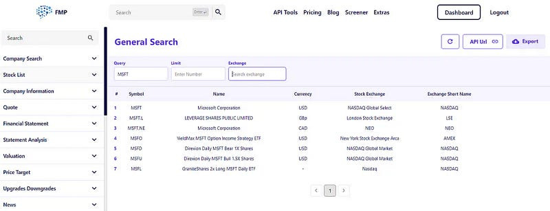
FMP stock price API is in real time, the company reports can be found in quarter or annual format, and goes up to 30 years back in history. The interface is extremely user-friendly and has the following appearance:
On the left, the tab lets you choose the different elements such as sentiment analysis and historical data. In the middle, you have the search bar for the asset, and on the right, you have the export option to download the required data.
Go to Charts → Daily Chart EOD, then write Apple in the search bar and select the start period of historical data (I’ve chosen 2000 to have a lot of historical data). Then, apply and export as csv.
Financial Modeling Prep - FinancialModelingPrep
FMP offers a stock market data API covers real-time stock prices, historical prices and market news to stock…site.financialmodelingprep.com
Clean the excel file by keeping only the close price and adjusting the dates to become descending rather than ascending and save as an excel workbook file.
Creating the Algorithm
Let’s start coding the algorithm. The next step is to calculate the price differences of Apple’s stock. This makes the time series stationary and better suited for machine learning models (in this case, it is rather a deep learning model as LSTMs are slightly more complex to be put with machine learning models). Use the following code:
# Importing libraries
from keras.models import Sequential
from keras.layers import Dense, LSTM
import keras
import numpy as np
import matplotlib.pyplot as plt
import pandas as pd

def volatility(data, lookback, close, position):
    data = add_column(data, 1)
    for i in range(len(data)):
        try:
            data[i, position] = (data[i - lookback + 1:i + 1, close].std())
        except IndexError:
            pass
    data = delete_row(data, lookback)
    return data

def add_column(data, times):
    for i in range(1, times + 1):
        new = np.zeros((len(data), 1), dtype = float)
        data = np.append(data, new, axis = 1)
    return data

def delete_row(data, number):
    data = data[number:, ]
    return data

# Importing the data
data = pd.read_excel('APPLE.xlsx').values

# Difference the data and make it stationary
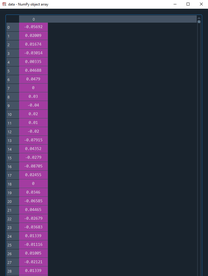
data = np.reshape(np.diff(data[:, 0]), (-1, 1))

# Calculating a rolling standard deviation on the returns
data = volatility(data, 20, 0, 1)

# Calculate the change in volatility
data = np.reshape(np.diff(data[:, 1]), (-1, 1))Financial Modeling Prep - FinancialModelingPrep
FMP offers a stock market data API covers real-time stock prices, historical prices and market news to stock…site.financialmodelingprep.com
The next step is to split the data and choose the hyperparameters. But wait, what are hyperparameters? Hyperparameters are the parameters set before the learning process begins and control the behavior and performance of the LSTM model. These parameters are not learned from the data; instead, they need to be defined and optimized by the user.
# Setting the hyperparameters
num_lags = 100
train_test_split = 0.80
num_neurons_in_hidden_layers = 20
num_epochs = 100
batch_size = 32

def data_preprocessing(data, num_lags, train_test_split):
    # Prepare the data for training
    x = []
    y = []
    for i in range(len(data) - num_lags):
        x.append(data[i:i + num_lags])
        y.append(data[i+ num_lags])
    # Convert the data to numpy arrays
    x = np.array(x)
    y = np.array(y)
    # Split the data into training and testing sets
    split_index = int(train_test_split * len(x))
    x_train = x[:split_index]
    y_train = y[:split_index]
    x_test = x[split_index:]
    y_test = y[split_index:]

    return x_train, y_train, x_test, y_test

# Creating the training and test sets
x_train, y_train, x_test, y_test = data_preprocessing(data, num_lags, train_test_split)

# Reshape the data for LSTM input
x_train = x_train.reshape((-1, num_lags, 1))
x_test = x_test.reshape((-1, num_lags, 1))
Next, fit the model to the training set as follows:
# Create the LSTM model
model = Sequential()

# First LSTM layer
model.add(LSTM(units = num_neurons_in_hidden_layers, input_shape = (num_lags, 1)))

# Second hidden layer
model.add(Dense(num_neurons_in_hidden_layers, activation = 'relu'))

# Output layer
model.add(Dense(units = 1))

# Compile the model
model.compile(loss = 'mean_squared_error', optimizer = 'adam')

# Train the model
model.fit(x_train, y_train, epochs = num_epochs , batch_size = batch_size)

# Predicting in-sample
y_predicted_train = np.reshape(model.predict(x_train), (-1, 1))

# Predicting out-of-sample
y_predicted = np.reshape(model.predict(x_test), (-1, 1))
And finally, plot the results and evaluate the performance using the accuracy metric (the hit ratio). Remember, the aim is to predict the change in volatility of Apple’s stock return. Hence, we can have either a positive or a negative value. The key objective is to be right most of the time. This is easier said than done of course.
def plot_train_test_values(window, train_window, y_train, y_test, y_predicted):
    prediction_window = window
    first = train_window
    second = window - first
    y_predicted = np.reshape(y_predicted, (-1, 1))
    y_test = np.reshape(y_test, (-1, 1))
    plotting_time_series = np.zeros((prediction_window, 3))
    plotting_time_series[0:first, 0] = y_train[-first:]
    plotting_time_series[first:, 1] = y_test[0:second, 0]
    plotting_time_series[first:, 2] = y_predicted[0:second, 0]
    plotting_time_series[0:first, 1] = plotting_time_series[0:first, 1] / 0
    plotting_time_series[0:first, 2] = plotting_time_series[0:first, 2] / 0
    plotting_time_series[first:, 0] = plotting_time_series[first:, 0] / 0
    plt.plot(plotting_time_series[:, 0], label = 'Training data', color = 'black', linewidth = 2.5)
    plt.plot(plotting_time_series[:, 1], label = 'Test data', color = 'black', linestyle = 'dashed', linewidth = 2)
    plt.plot(plotting_time_series[:, 2], label = 'Predicted data', color = 'red', linewidth = 1)
    plt.axvline(x = first, color = 'black', linestyle = '--', linewidth = 1)
    plt.grid()
    plt.legend()

def calculate_accuracy(predicted_returns, real_returns):
    predicted_returns = np.reshape(predicted_returns, (-1, 1))
    real_returns = np.reshape(real_returns, (-1, 1))
    hits = sum((np.sign(predicted_returns)) == np.sign(real_returns))
    total_samples = len(predicted_returns)
    accuracy = hits / total_samples

    return accuracy[0] * 100

# Plotting
y_train = np.reshape(y_train, (-1))
plot_train_test_values(100, 50, y_train, y_test, y_predicted)

# Performance evaluation
print('---')
print('Accuracy Train = ', round(calculate_accuracy(y_predicted_train, y_train), 2), '%')
print('Accuracy Test = ', round(calculate_accuracy(y_predicted, y_test), 2), '%')
print('---')---
Accuracy Train = 51.46 %
Accuracy Test = 50.76 %
---In conclusion, you can always try to be creative with your algorithms and seek to analyze complex and exotic data in search of predictability.
You can also check out my other newsletter The Weekly Market Sentiment Report that sends weekly directional views every weekend to highlight the important trading opportunities using a mix between sentiment analysis (COT report, put-call ratio, etc.) and rules-based technical analysis.
If you liked this article, do not hesitate to like and comment, to further the discussion!


