
Use this Reversal Strategy in Your Trading
Creating a Double Reversal Strategy Using the RSI & Stochastic


This article discusses an interesting strategy based on two methods and two indicators. The aim is to find reversal signals that are used for medium-term extended periods.
I have released a new book called “Contrarian Trading Strategies in Python”. It features a lot of advanced contrarian indicators and strategies with a GitHub page dedicated to the continuously updated code. If you are interested, you could buy the PDF version directly through a PayPal payment of 9.99 EUR.
Please include your email in the note before paying so that you receive it on the right address. Also, once you receive it, make sure to download it through google drive.
Pay Kaabar using PayPal.Me
If you accept cookies, we’ll use them to improve and customize your experience and enable our partners to show you…www.paypal.com
The Relative Strength Index
First introduced by J. Welles Wilder Jr., the RSI is one of the most popular and versatile technical indicators. Mainly used as a contrarian indicator where extreme values signal a reaction that can be exploited. Typically, we use the following steps to calculate the default RSI:
Calculate the change in the closing prices from the previous ones.
Separate the positive net changes from the negative net changes.
Calculate a smoothed moving average on the positive net changes and on the absolute values of the negative net changes.
Divide the smoothed positive changes by the smoothed negative changes. We will refer to this calculation as the Relative Strength — RS.
Apply the normalization formula shown below for every time step to get the RSI.


The above chart shows the hourly values of the GBPUSD in black with the 13-period RSI. We can generally note that the RSI tends to bounce close to 25 while it tends to pause around 75. To code the RSI in Python, we need an OHLC array composed of four columns that cover open, high, low, and close prices.
def add_column(data, times):

    for i in range(1, times + 1):

        new = np.zeros((len(data), 1), dtype = float)

        data = np.append(data, new, axis = 1)
return datadef delete_column(data, index, times):
for i in range(1, times + 1):
data = np.delete(data, index, axis = 1) return datadef delete_row(data, number):
data = data[number:, ]
return datadef ma(data, lookback, close, position):
data = add_column(data, 1)
for i in range(len(data)):
try:
data[i, position] = (data[i - lookback + 1:i + 1, close].mean())
except IndexError:
pass
data = delete_row(data, lookback)
return datadef smoothed_ma(data, alpha, lookback, close, position):
lookback = (2 * lookback) - 1
alpha = alpha / (lookback + 1.0)
beta = 1 - alpha
data = ma(data, lookback, close, position) data[lookback + 1, position] = (data[lookback + 1, close] * alpha) + (data[lookback, position] * beta) for i in range(lookback + 2, len(data)):
try:
data[i, position] = (data[i, close] * alpha) + (data[i - 1, position] * beta)
except IndexError:
pass
return datadef rsi(data, lookback, close, position):
data = add_column(data, 5)
for i in range(len(data)):
data[i, position] = data[i, close] - data[i - 1, close]
for i in range(len(data)):
if data[i, position] > 0:
data[i, position + 1] = data[i, position]
elif data[i, position] < 0:
data[i, position + 2] = abs(data[i, position])
data = smoothed_ma(data, 2, lookback, position + 1, position + 3)
data = smoothed_ma(data, 2, lookback, position + 2, position + 4) data[:, position + 5] = data[:, position + 3] / data[:, position + 4]
data[:, position + 6] = (100 - (100 / (1 + data[:, position + 5]))) data = delete_column(data, position, 6)
data = delete_row(data, lookback) return dataMake sure to focus on the concepts and not the code. You can find the codes of most of my strategies in my books. The most important thing is to comprehend the techniques and strategies.
The Stochastic Oscillator
The stochastic oscillator seeks to find oversold and overbought zones by incorporating the highs and lows using a normalization formula as shown below:

An overbought level is an area where the market is perceived to be extremely bullish and is bound to consolidate. An oversold level is an area where market is perceived to be extremely bearish and is bound to bounce. Hence, the stochastic oscillator is a contrarian indicator that seeks to signal reactions of extreme movements. We will create the below function that calculates the stochastic on an OHLC data:
def stochastic_oscillator(data,
                             lookback,
                             high,
                             low,
                             close,
                             where,
                             slowing = False,
                             smoothing = False,
                             slowing_period = 1,
                             smoothing_period = 1):

    data = adder(data, 1)

    for i in range(len(data)):

        try:

            data[i, where] = (data[i, close] - min(data[i - lookback + 1:i + 1, low])) / (max(data[i - lookback + 1:i + 1, high]) - min(data[i - lookback + 1:i + 1, low]))

        except ValueError:

            pass

    data[:, where] = data[:, where] * 100

    if slowing == True and smoothing == False:

        data = ma(data, slowing_period, where, where + 1)

    if smoothing == True and slowing == False:

        data = ma(data, smoothing_period, where, where + 1)

    if smoothing == True and slowing == True:

        data = ma(data, slowing_period, where,   where + 1)

        data = ma(data, smoothing_period, where, where + 2)

    data = jump(data, lookback)

    return data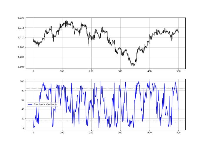
my_data = stochastic_oscillator(my_data,
                             100,
                             1,
                             2,
                             3,
                             5,
                             slowing = True,
                             smoothing = False,
                             slowing_period = 3,
                             smoothing_period = 1)
# my_data must be an OHLC array with four columns composed of open, high, low, and close pricesMake sure to focus on the concepts and not the code. The most important thing is to comprehend the techniques and strategies. The code is a matter of execution but the idea is something you cook in your head for a while.
Check out my weekly market sentiment report to understand the current positioning and to estimate the future direction of several major markets through complex and simple models working side by side. Find out more about the report through this link:
Coalescence Report 1st May — 8th May 2022
This report covers the weekly market sentiment and positioning and any changes that have occurred which might present…coalescence.substack.com
Creating the Strategy
The strategy has rare signals but they are generally of higher quality than plain vanilla indicators. We will look for a normal divergence on a 13-period RSI while the 100-period stochastic oscillator is around the extreme levels. The following are the details:
Long (Buy) whenever the 100-period stochastic oscillator is below 20 while the RSI has just confirmed a bullish divergence.
Short (Sell) whenever the 100-period stochastic oscillator is above 80 while the RSI has just confirmed a bearish divergence.
Naturally, when prices are rising and making new tops while a price-based indicator is making lower tops, a weakening is occurring and a possibility to change the bias from long to short can present itself. That is what we call a normal divergence. We know that:
When prices are making higher highs while the indicator is making lower highs, it is called a bearish divergence, and the market might stall.
When prices are making lower lows while the indicator is making higher lows, it is called a bullish divergence, and the market might show some upside potential.

def divergence(Data, indicator, lower_barrier, upper_barrier, width, buy, sell):
    Data = adder(Data, 2)
    for i in range(len(Data)):
        try:
            if Data[i, indicator] < lower_barrier:
                for a in range(i + 1, i + width):
                    if Data[a, indicator] > lower_barrier:
                        for r in range(a + 1, a + width):
                            if Data[r, indicator] < lower_barrier and \
                            Data[r, indicator] > Data[i, indicator] and Data[r, 3] < Data[i, 3]:
                                for s in range(r + 1, r + width):
                                    if Data[s, indicator] > lower_barrier:
                                        Data[s, buy] = 1
                                        break
                                    else:
                                        break
                            else:
                                break
                        else:
                            break
                    else:
                        break
        except IndexError:
            pass
    for i in range(len(Data)):
        try:
            if Data[i, indicator] > upper_barrier:
                for a in range(i + 1, i + width):
                    if Data[a, indicator] < upper_barrier:
                        for r in range(a + 1, a + width):
                            if Data[r, indicator] > upper_barrier and \
                            Data[r, indicator] < Data[i, indicator] and Data[r, 3] > Data[i, 3]:
                                for s in range(r + 1, r + width):
                                    if Data[s, indicator] < upper_barrier:
                                        Data[s, sell] = -1
                                        break
                                    else:
                                        break
                            else:
                                break
                        else:
                            break
                    else:
                        break
        except IndexError:
            pass
    return Data
The signal charts show the moment a divergence is validated while the stochastic oscillator is showing extreme readings.

def signal(data, stochastic_column, bull_divergence, column, bear_divergence, buy, sell):data = adder(data, 5)for i in range(len(data)):
if data[i, bull_divergence] == 1 and data[i, stochastic_column] < 20:
data[i, buy] = 1
if data[i, bear_divergence] == -1 and data[i, stochastic_column] > 80:
data[i, sell] = -1
return data
Summary
To sum up, what I am trying to do is to simply contribute to the world of objective technical analysis which is promoting more transparent techniques and strategies that need to be back-tested before being implemented. This way, technical analysis will get rid of the bad reputation of being subjective and scientifically unfounded.
I recommend you always follow the the below steps whenever you come across a trading technique or strategy:
Have a critical mindset and get rid of any emotions.
Back-test it using real life simulation and conditions.
If you find potential, try optimizing it and running a forward test.
Always include transaction costs and any slippage simulation in your tests.
Always include risk management and position sizing in your tests.
Finally, even after making sure of the above, stay careful and monitor the strategy because market dynamics may shift and make the strategy unprofitable.