Unlocking Time Series Secrets With ARIMA
A Comprehensive Guide to Understanding and Implementing ARIMA
Widely used for time series analysis, ARIMA models combine autoregression, differencing, and moving averages to make accurate observations based on historical data. This article demystifies the ARIMA model, providing you with essential insights, practical applications, and a step-by-step guide to mastering time series in Python.
The Foundations of ARIMA
ARIMA stands for autoregressive integrated moving average. It is a popular and widely used statistical model for analyzing and forecasting time series data. The ARIMA model combines three key components: autoregression (AR), differencing (I for integrated), and moving average (MA). In further details, it is as follows:
The autoregressive part (AR) of the model specifies that the output variable depends linearly on its own previous values. It is denoted by p, which is the number of lag observations included in the model.
The integrated part (I) of the model involves differencing the data series to make it stationary. Stationarity implies that the properties of the series do not depend on the time at which the series is observed. It is denoted by d, which is the number of times the raw observations are differenced.
The moving average part (MA) specifies that the output variable depends linearly on the past error terms. It is denoted by q, which is the size of the moving average window.
Hence, the ARIMA model is simply a function of p, q, and d:
The three above parameters are determined in the data preparation step by using the autocorrelation function (ACF) and the partial autocorrelation function (PACF). How is this done? Well, first let’s define both functions:
The autocorrelation function (ACF) measures the correlation between observations of a time series separated by different time lags. It helps in identifying the strength and direction of the relationship between the observations at different lags. A gradual decline in autocorrelations (i.e., “decay”) suggests non-stationarity in the series.
Significant spikes in the ACF plot indicate strong correlations at specific lags.
The partial autocorrelation function (PACF) measures the correlation between observations of a time series separated by a certain lag, controlling for the values of the time series at shorter lags. It helps in identifying the direct effect of a lag on the series, without the influence of shorter lags. A sharp drop after a few lags suggests a cut-off point, indicating the order of the autoregressive part.
Significant spikes in the PACF plot indicate the lags that have a direct effect on the series.
The parameter d represents the number of differences needed to make the time series stationary (generally, it is 1). A stationary series has a constant mean and variance over time. To check for stationarity, we can use the ADF test.
The parameter p represents the number of lag observations included in the model. We have to look for the lag at which the PACF plot cuts off sharply (i.e., where the partial autocorrelations become insignificant). This lag suggests the order of the autoregressive part.
The parameter q represents the size of the moving average window. Look for the lag at which the ACF plot cuts off sharply (i.e., where the autocorrelations become insignificant). This lag suggests the order of the moving average part.
Check out my newsletter that sends weekly directional views every weekend to highlight the important trading opportunities using a mix between sentiment analysis (COT report, put-call ratio, etc.) and rules-based technical analysis.
Coding ARIMA in Python
Let’s take an example to clarify all of this. We will generate a synthetic time series, calculate the three parameters, apply the ARIMA model and forecast the future values. Use the following code:
import pandas as pd
import numpy as np
import matplotlib.pyplot as plt
from statsmodels.graphics.tsaplots import plot_acf, plot_pacf
from statsmodels.tsa.arima.model import ARIMA
from statsmodels.tsa.stattools import adfuller

# Generate synthetic data
date_range = pd.date_range(start="2020-01-01", periods=365, freq="D")
data = pd.DataFrame({
    "date": date_range,
    "value": np.sin(np.arange(len(date_range)) * 2 * np.pi / 30) + np.random.normal(0, 0.1, size=len(date_range))
})
data.set_index("date", inplace=True)
# Plot the data
plt.figure(figsize=(10, 6))
plt.plot(data, color = 'black')
plt.title("Synthetic Time Series Data")
plt.legend()
plt.show()
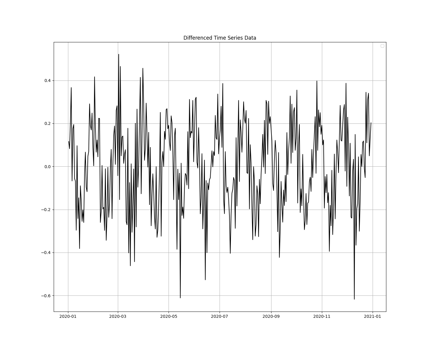
plt.grid()Next, check for the stationarity of the above data. If the p-value is greater than 0.05, then it is not stationary. Afterwards, difference the data, to make it stationary and plot the new graph:
# Check for stationarity using the Augmented Dickey-Fuller test
result = adfuller(data['value'])
print('ADF Statistic:', result[0])
print('p-value:', result[1])
print('Critical Values:', result[4])

# If non-stationary, difference the data
data_diff = data['value'].diff().dropna()
# Plot differenced data
plt.figure(figsize=(10, 6))
plt.plot(data_diff, color = 'black')
plt.title("Differenced Time Series Data")
plt.legend()
plt.show()
plt.grid()Plot the ACF and PACD graphs:
# Plot ACF and PACF to identify p and q
fig, axes = plt.subplots(1, 2, figsize=(15, 6))
plot_acf(data_diff, ax=axes[0])
plot_pacf(data_diff, ax=axes[1])
plt.show()Fit and predict using ARIMA:
# Define the ARIMA model with identified parameters (example: p=1, d=1, q=1)
model = ARIMA(data['value'], order=(1, 1, 1))
model_fit = model.fit()

# Print model summary
print(model_fit.summary())
# Forecast
forecast = model_fit.forecast(steps=30)
forecast_index = pd.date_range(start=data.index[-1] + pd.Timedelta(days=1), periods=30, freq="D")
# Plot the forecast
plt.figure(figsize=(10, 6))
plt.plot(data['value'], color = 'black', label='Original Data')
plt.plot(forecast_index, forecast, label='Forecast', color='red')
plt.title("ARIMA Forecast")
plt.legend()
plt.show()
plt.grid()
Obviously, ARIMA (1, 1, 1) comes from the fact that we differenced the data once, and the ACF/PCF cut off sharply at 1.
Throughout this article, we explored the theoretical foundations of ARIMA, delving into its autoregressive, differencing, and moving average components. We also demonstrated how to implement ARIMA models in Python using the statsmodels library, providing a practical, step-by-step guide to building and interpreting these models.


