Understanding Logistic Regression - A Step-by-Step Tutorial
Understanding the Logic: A Deep Dive into Logistic Regression Concepts
This article is a down-to-earth guide on logistic regression, cutting through the technical jargon to explain the method’s nuts and bolts. We’ll walk through the basics, from understanding the sigmoid function to making sense of those coefficients. Whether you’re just starting with data science or want a refresher on logistic regression, this guide is here to demystify the process and make it practical for your time series projects.
Introduction to Logistic Regression
Logistic regression is a statistical method used for binary classification tasks, where the outcome variable is categorical and has two classes (0 and 1). It’s an extension of linear regression but adapted for predicting the probability of an observation belonging to one of the two classes.
In logistic regression, the logistic function (also called the sigmoid function) is used to map the linear combination of input features to a probability between 0 and 1.
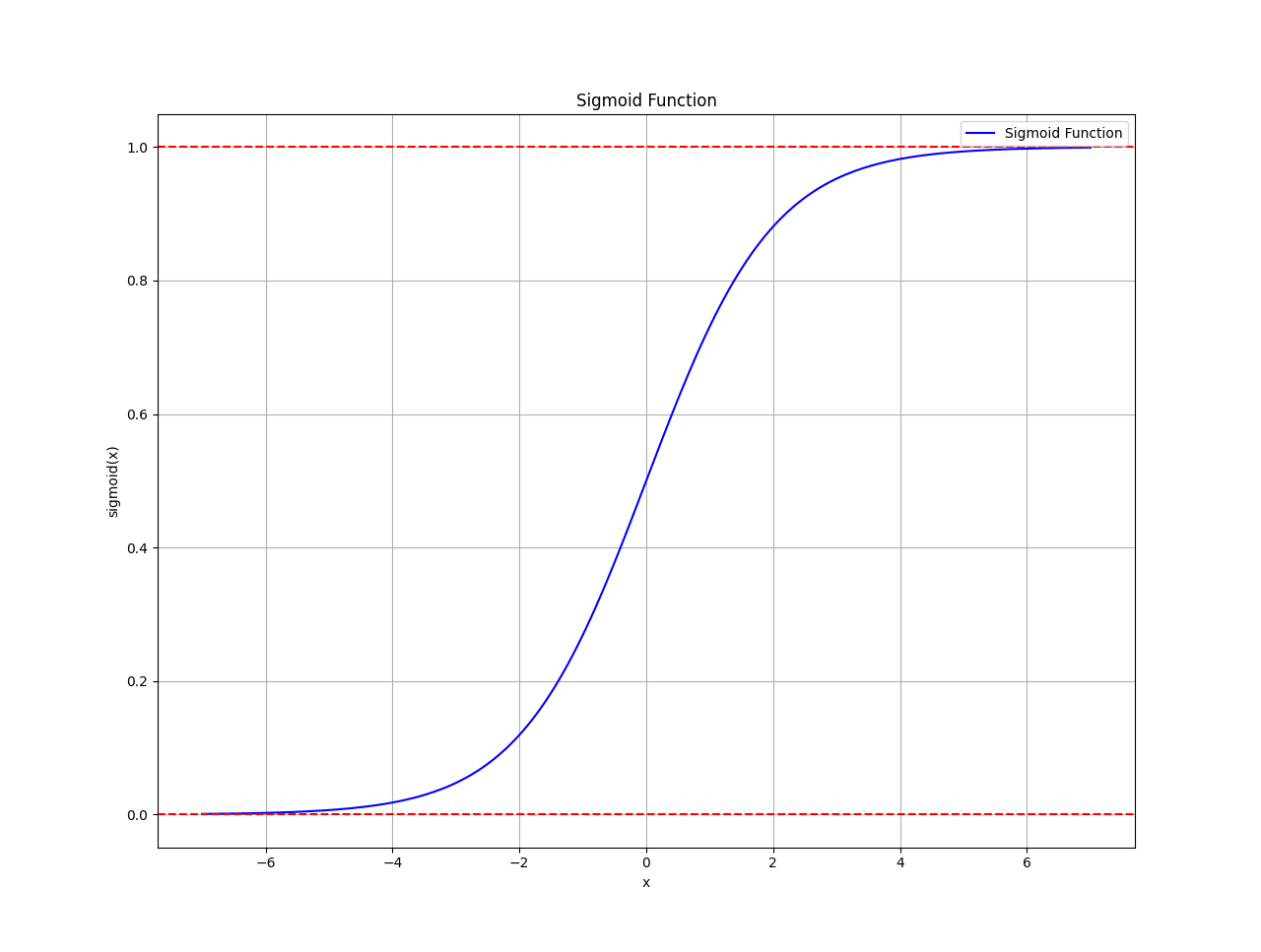
The sigmoid function, also known as the logistic function, is a mathematical function that maps any real-valued number to a value between 0 and 1. It’s characterized by its S-shaped curve, which is why it’s often referred to as an “S-curve.”
The sigmoid function is defined by the following formula:
The following chart shows the Sigmoid function.
To plot the previous chart, you can use the following code:
import numpy as np
import matplotlib.pyplot as plt

# Define the sigmoid function
def sigmoid(x):
    return 1 / (1 + np.exp(-x))
# Generate x values
x_values = np.linspace(-7, 7, 200)
# Calculate corresponding y values using the sigmoid function
y_values = sigmoid(x_values)
# Plot the sigmoid function
plt.figure(figsize=(8, 6))
plt.plot(x_values, y_values, label='Sigmoid Function', color='blue')
plt.title('Sigmoid Function')
plt.xlabel('x')
plt.ylabel('sigmoid(x)')
plt.axhline(0, color='red', linestyle='--')
plt.axhline(1, color='red', linestyle='--')
plt.legend()
plt.grid(True)
plt.show()
The logic behind logistic regression lies in modeling the probability of an event occurring, given a set of input features.
If you want to see more of my work, you can visit my website for the books catalogue by simply following this link:
Creating the Algorithm
The aim of the algorithm is to run an autoregressive logistic task on the binary changes in the S&P 500 index (1’s for when it goes up and 0’s for when it goes down). For this task, we can follow this framework:
Import the file to Python and split it into a training set and a test set.
Select the lags that will be used to forecast the current values, then fit and predict the model.
Evaluate the model and plot the results.
from sklearn.linear_model import LogisticRegression
from sklearn.metrics import accuracy_score
import pandas_datareader as pdr
import numpy as np

def data_preprocessing(data, num_lags, train_test_split):
    # Prepare the data for training
    x = []
    y = []
    for i in range(len(data) - num_lags):
        x.append(data[i:i + num_lags])
        y.append(data[i+ num_lags])
    # Convert the data to numpy arrays
    x = np.array(x)
    y = np.array(y)
    # Split the data into training and testing sets
    split_index = int(train_test_split * len(x))
    x_train = x[:split_index]
    y_train = y[:split_index]
    x_test = x[split_index:]
    y_test = y[split_index:]

    return x_train, y_train, x_test, y_test
start_date = '1960-01-01'
end_date   = '2020-01-01'
# Set the time index if it's not already set
data = (pdr.get_data_fred('SP500', start = start_date, end = end_date).dropna())
data = np.reshape(data, (-1))
data = np.diff(data)
data = np.where(data > 0, 1, 0)
# Train-test split
x_train, y_train, x_test, y_test = data_preprocessing(data, 100, 0.80)
# Create and train the logistic regression model
model = LogisticRegression()
model.fit(x_train, y_train)
# Make predictions on the test set
predictions = model.predict(x_test)
# Evaluate the model
accuracy = accuracy_score(y_test, predictions)
print(f"Accuracy: {accuracy}")
The output of the code is as follows:
Accuracy: 0.5400696864111498The logic behind logistic regression involves transforming a linear combination of input features into probabilities using the sigmoid function. The model is trained to maximize the likelihood of the observed outcomes, and the resulting coefficients allow for interpreting the impact of each feature on the probability of the event occurring. The decision boundary and threshold determine the classification of observations into two classes.
You can also check out my other newsletter The Weekly Market Sentiment Report that sends weekly directional views every weekend to highlight the important trading opportunities using a mix between sentiment analysis (COT report, put-call ratio, etc.) and rules-based technical analysis.
If you liked this article, do not hesitate to like and comment, to further the discussion!


