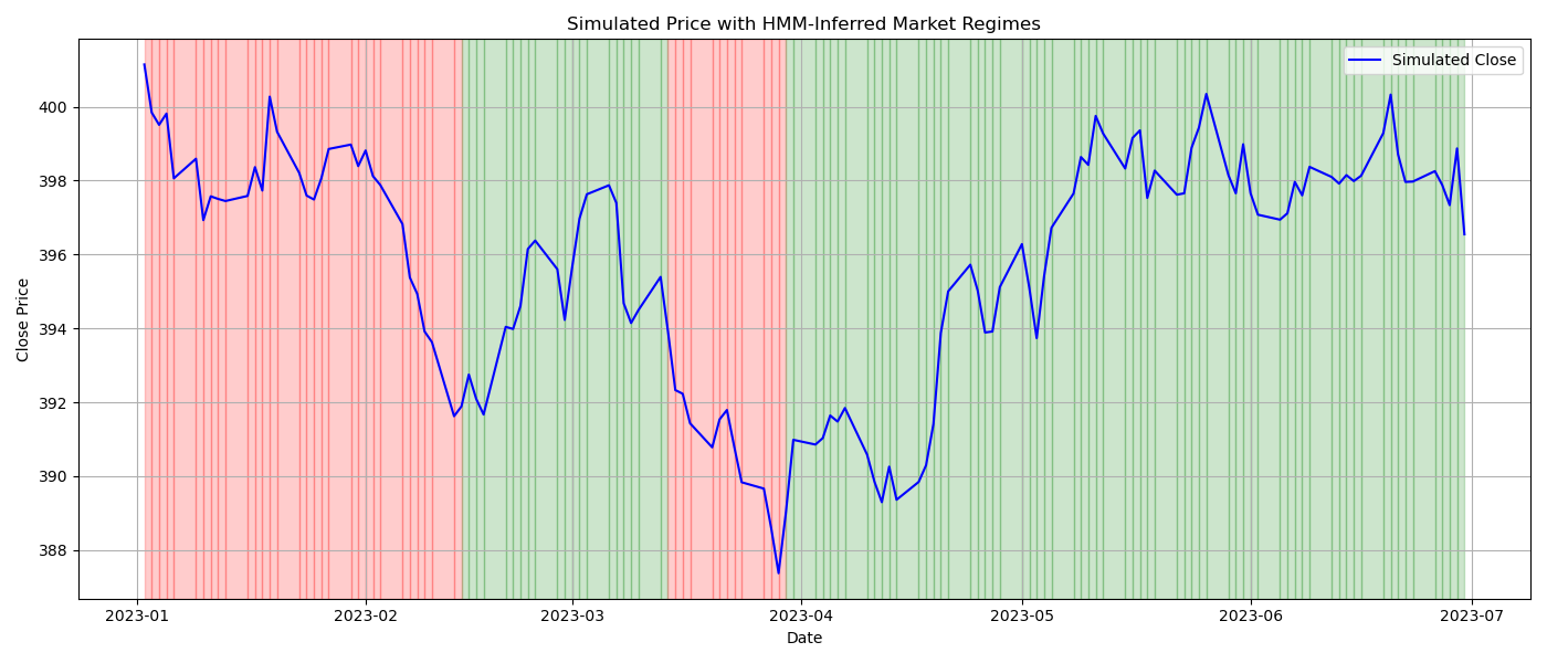
Let’s get something straight: Hidden Markov Models (HMMs) sound more complicated than they are. If you’ve ever made a guess about something you couldn’t see—like what mood your friend is in based on their tone of voice—you’re already doing a kind of HMM reasoning.
In this post, we’ll break HMMs down like a puzzle:
What they are (with real-world examples)
Why they’re powerful
How they work under the hood
And how to implement them in Python from scratch with regards to time series
What Is a Hidden Markov Model?
A Hidden Markov Model (HMM) is a statistical model where:
There’s an underlying system you can’t directly observe (these are the hidden states).
You can observe outputs that are influenced by these hidden states (these are the emissions or observations).
The hidden states evolve over time, and the way they transition follows a Markov process — which means the future state depends only on the current one, not the whole past.
Markets are complex, but patterns repeat. We often talk about:
Bull markets (prices generally rising)
Bear markets (prices generally falling)
But you can’t see the regime directly. You only see what the market does: price movements, volatility, volume. These are observations. The underlying regime is hidden — but it drives those observations. That’s exactly what HMMs are built for.
Imagine you’re trying to guess the weather (sunny or rainy) based on your friend’s activity (walking, shopping, or cleaning). You can’t see the weather directly, but you see what your friend does. Over time, you notice patterns:
If it’s sunny, your friend often goes walking.
If it’s rainy, they’re more likely to clean or shop indoors.
You can build an HMM to learn and infer the most likely weather pattern over a week of observed behaviors.
An HMM has:
States (hidden):
These are the things you can’t directly observe.
Example:
[”Sunny”, “Rainy”]
Observations:
These are what you can see.
Example:
[”Walk”, “Shop”, “Clean”]
Transition probabilities:
Probability of moving from one hidden state to another.
Example:
P(Sunny → Rainy) = 0.3
Emission probabilities:
Probability of an observation given a hidden state.
Example:
P(Walk | Sunny) = 0.6
Initial probabilities:
How likely each hidden state is at the start.
Example:
P(Sunny) = 0.5
The Goal: Regime Detection from Daily Price Moves
From the section’s name, you understand that we’re trying to infer the market regime from daily price moves. For this, we would like to visualize on a time series of our choice a bullish regime in green and a bearish regime in red as the following chart shows.
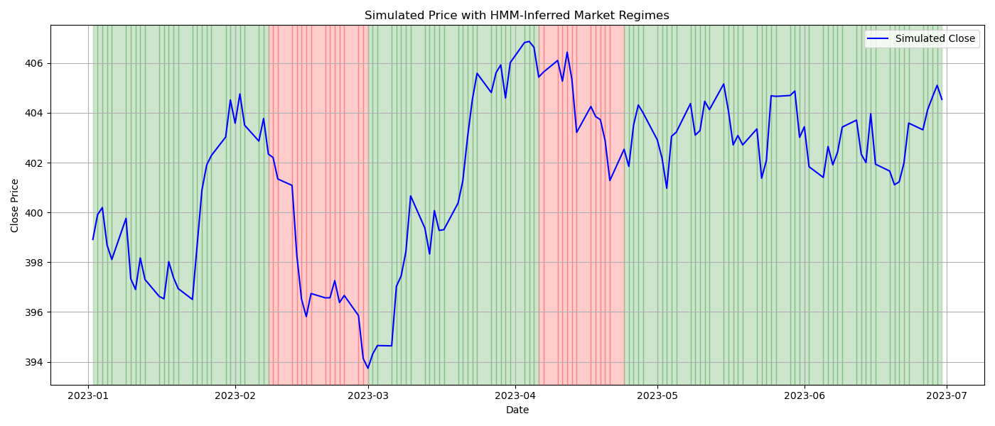
To do this experiment, we can use the following code:
import numpy as np
import pandas as pd
import matplotlib.pyplot as plt
import datetime

# Generate synthetic daily prices and returns
np.random.seed(455)
dates = pd.date_range(start=”2023-01-01”, end=”2023-06-30”, freq=’B’)  # Business days
n_days = len(dates)
prices = 400 + np.cumsum(np.random.normal(0, 1, size=n_days))  # Simulated prices
returns = np.diff(prices) / prices[:-1]
returns = np.insert(returns, 0, 0)  # First return is 0

# Categorize returns
def categorize(r, threshold=0.002):
    if r > threshold:
        return “Up”
    elif r < -threshold:
        return “Down”
    else:
        return “Flat”

movements = [categorize(r, threshold=0.002) for r in returns]

# Create the DataFrame
data = pd.DataFrame({
    “Date”: dates,
    “Adj Close”: prices,
    “Return”: returns,
    “Movement”: movements
})

# HMM Setup
states = [”Bull”, “Bear”]
obs_set = [”Up”, “Flat”, “Down”]
obs_map = {o: i for i, o in enumerate(obs_set)}
obs_seq = [obs_map[o] for o in data[’Movement’]]

start_prob = np.array([0.6, 0.4])
trans_prob = np.array([
    [0.90, 0.10],  # Bull -> Bull, Bear
    [0.20, 0.80],  # Bear -> Bull, Bear
])
emiss_prob = np.array([
    [0.70, 0.10, 0.20],  # Bull: Up, Flat, Down
    [0.20, 0.10, 0.70],  # Bear: Up, Flat, Down
])

# Viterbi algorithm
def viterbi(obs_seq, states, start_p, trans_p, emiss_p):
    T = len(obs_seq)
    N = len(states)
    dp = np.zeros((N, T))
    backptr = np.zeros((N, T), dtype=int)
    dp[:, 0] = start_p * emiss_p[:, obs_seq[0]]

    for t in range(1, T):
        for s in range(N):
            probs = dp[:, t-1] * trans_p[:, s] * emiss_p[s, obs_seq[t]]
            dp[s, t] = np.max(probs)
            backptr[s, t] = np.argmax(probs)

    best_last = np.argmax(dp[:, T-1])
    best_prob = dp[best_last, T-1]

    best_path = [best_last]
    for t in range(T-1, 0, -1):
        best_path.insert(0, backptr[best_path[0], t])

    state_path = [states[i] for i in best_path]
    return state_path, best_prob

decoded_states, prob = viterbi(obs_seq, states, start_prob, trans_prob, emiss_prob)

# Add to DataFrame
data[’Regime’] = decoded_states

# Plot
plt.figure(figsize=(14, 6))
plt.plot(data[’Date’], data[’Adj Close’], label=”Simulated Close”, color=’blue’)

# Regime shading
for i in range(len(data) - 1):
    start_date = data.loc[i, ‘Date’]
    end_date = data.loc[i + 1, ‘Date’]
    regime = data.loc[i, ‘Regime’]
    color = ‘green’ if regime == “Bull” else ‘red’
    plt.axvspan(start_date, end_date, color=color, alpha=0.2)

plt.xlabel(”Date”)
plt.ylabel(”Close Price”)
plt.title(”Simulated Price with HMM-Inferred Market Regimes”)
plt.legend()
plt.grid(True)
plt.tight_layout()
plt.show()
In layman’s terms, here’s what this whole HMM algorithm does:
You see the price go up, go down, or stay flat. That’s all you can see — just the outcomes. But beneath those movements, you suspect something deeper is going on — like the market being in a bullish mood (optimistic) or a bearish mood (pessimistic). You can’t see those moods directly. You can only guess them based on what the market does. What the HMM does is:
It uses math to guess the most likely sequence of hidden moods (regimes) behind the market’s daily behavior.
It answers: Given these ups and downs in the stock price, what’s the most likely sequence of bull and bear markets that explains them?
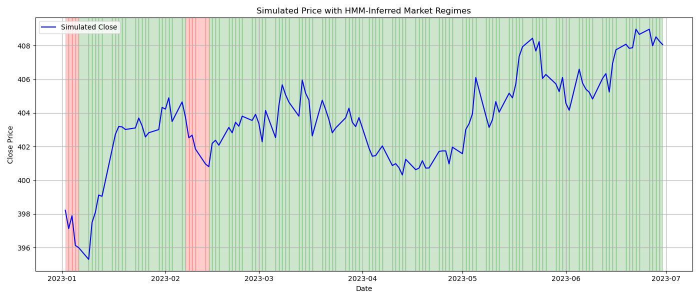
It works in 3 basic steps:
Set the Rules: You give it some general rules about how bull and bear markets behave:
Bull markets: mostly go up.
Bear markets: mostly go down.
Markets don’t switch moods too often.
Look at the Data: You feed in a sequence of actual daily movements (up, down, flat).
Decode the Mood: The algorithm runs through the entire sequence and figures out, day by day:
“Was the market probably in a bull or bear mood on this day?”
It does this using a smart path-finding trick (called the Viterbi algorithm) that balances the probabilities of state switches and daily behaviors.
This algorithm helps you see the hidden mood of the market using only the movements you can observe. It gives you a probabilistic guess at what’s going on under the surface.
The Viterbi algorithm works by evaluating every possible path of hidden states and efficiently selecting the one that best explains the observed data. It doesn’t just look at each day in isolation; it considers the entire sequence, using prior knowledge about state transitions and observable outcomes. In essence, it’s a way to reverse-engineer the most plausible underlying story from what you can see on the surface.