


The Stochastic Keltner Trading Strategy in Python
Creating and Back-testing a Contrarian Trading Strategy in Python


This article discusses a trading strategy based on the stochastic oscillator and the Keltner channel, a known volatility indicator. The strategy’s type is contrarian and is best used in ranging markets. The second part of the article will deal with performance evaluation on a selected sample of markets.
The Stochastic Oscillator
The stochastic oscillator is a known bounded technical indicator based on the normalization function. It traps the high, low, and close prices between 0 and 100 so as we get a glance on overstretched markets.
The stochastic oscillator (raw version) is calculated as follows:
Subtract the current close from the lowest low during the last 14 periods. Let’s call this step one.
Subtract the highest high during the last 14 periods from he lowest low during the last 14 periods. Let’s call this step two.
Divide step one by step two and multiply by 100.
The result is the raw version of the stochastic oscillator. The function we can use to code the stochastic oscillator given a numpy OHLC array is as follows:
def stochastic_oscillator(data,
                             lookback,
                             high,
                             low,
                             close,
                             position,
                             slowing = False,
                             smoothing = False,
                             slowing_period = 1,
                             smoothing_period = 1):

    data = add_column(data, 1)

    for i in range(len(data)):

        try:

            data[i, position] = (data[i, close] - min(data[i - lookback + 1:i + 1, low])) / (max(data[i - lookback + 1:i + 1, high]) - min(data[i - lookback + 1:i + 1, low]))

        except ValueError:

            pass

    data[:, position] = data[:, position] * 100

    if slowing == True and smoothing == False:

        data = ma(data, slowing_period, position, position + 1)

    if smoothing == True and slowing == False:

        data = ma(data, smoothing_period, position, position + 1)

    if smoothing == True and slowing == True:

        data = ma(data, slowing_period, position,   position + 1)

        data = ma(data, smoothing_period, position + 1, position + 2)

    data = delete_row(data, lookback)

    return data
You need to define the primal function first which are needed to make the function work. They are as follows:
def add_column(data, times):
for i in range(1, times + 1):
new = np.zeros((len(data), 1), dtype = float)
data = np.append(data, new, axis = 1)
return data
def delete_column(data, index, times):
for i in range(1, times + 1):
data = np.delete(data, index, axis = 1)
return data
def delete_row(data, number):
data = data[number:, ]
return data
def ma(data, lookback, close, position):
data = add_column(data, 1)
for i in range(len(data)):
try:
data[i, position] = (data[i - lookback + 1:i + 1, close].mean())
except IndexError:
pass
data = delete_row(data, lookback)
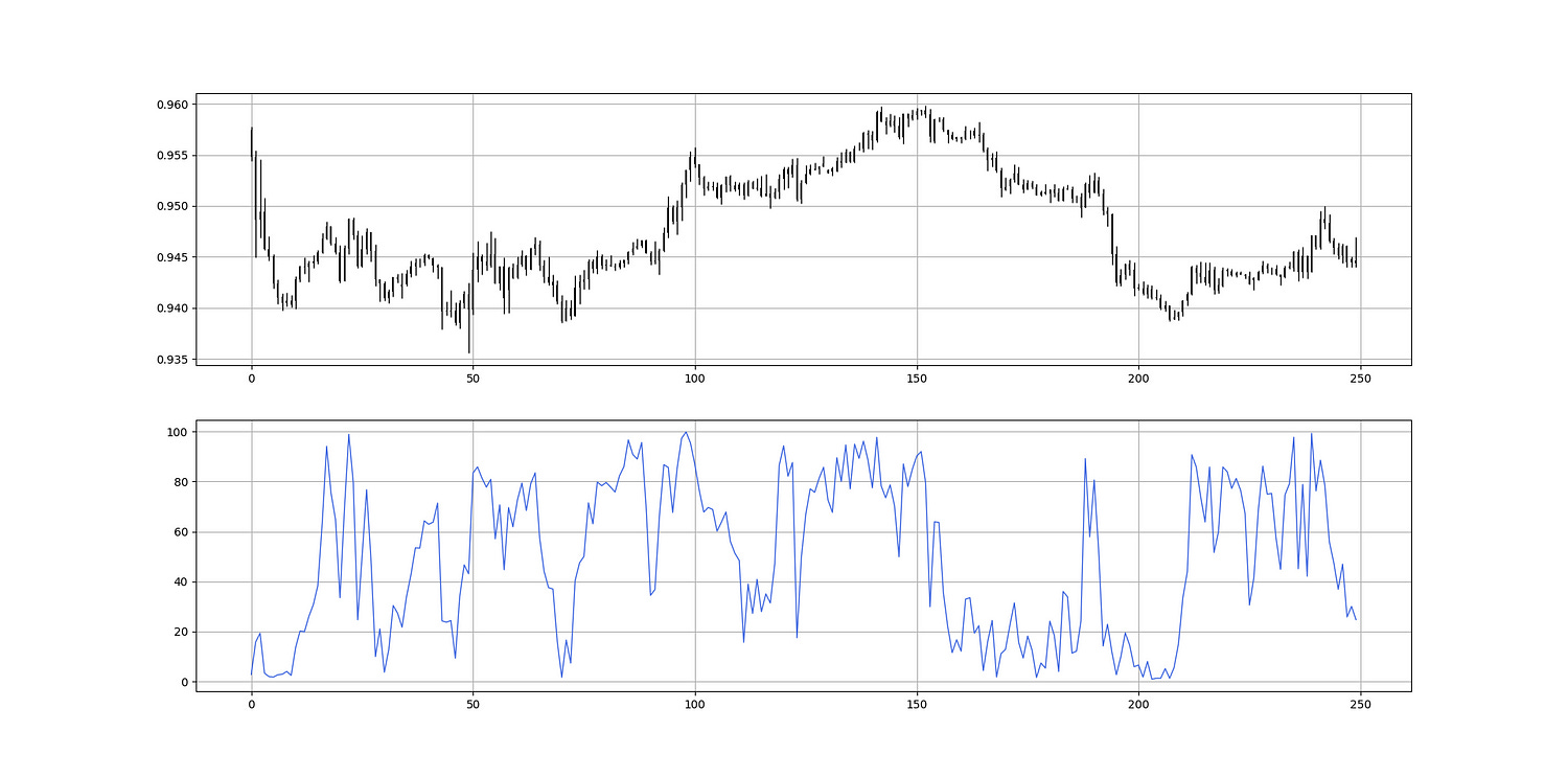
return dataAlso, make sure you have an array and not a data frame as the code exclusively works with arrays. The following Figure shows an example of the 14-period stochastic oscillator.
The Keltner Channel
The Keltner channel is a volatility bands indicator which tries to envelop the market price so as to find dynamic support and resistance levels. The steps used to calculate the Keltner channel are as follows:
Calculate an exponential moving average on the close prices.
Calculate an average true range (ATR) using the specified lookback period.
Add step one to step two and multiply by a constant.
Subtract step one from step two and multiply by a constant.
The function we can use to code the Keltner channel given a numpy OHLC array is as follows:
def keltner_channel(data, lookback, multiplier, close, position):

    data = add_column(data, 2)

    data = ema(data, 2, lookback, close, position)

    data = atr(data, lookback, 1, 2, 3, position + 1)

    data[:, position + 2] = data[:, position] + (data[:, position + 1] * multiplier)
    data[:, position + 3] = data[:, position] - (data[:, position + 1] * multiplier)

    data = delete_column(data, position, 2)
    data = delete_row(data, lookback)

    return data
You can also check out my other newsletter The Weekly Market Sentiment Report that sends tactical directional views every weekend to highlight the important trading opportunities using a mix between sentiment analysis (COT reports, Put-Call ratio, Gamma exposure index, etc.) and technical analysis.
Two additional functions must be defined for the above code to work and they are the functions of the Keltner channnel, smoothed moving average, and exponential moving average.
def ema(data, alpha, lookback, close, position):

    alpha = alpha / (lookback + 1.0)

    beta  = 1 - alpha

    data = ma(data, lookback, close, position)

    data[lookback + 1, position] = (data[lookback + 1, close] * alpha) + (data[lookback, position] * beta)

    for i in range(lookback + 2, len(data)):

            try:

                data[i, position] = (data[i, close] * alpha) + (data[i - 1, position] * beta)

            except IndexError:

                pass

    return data

def smoothed_ma(data, alpha, lookback, close, position):

    lookback = (2 * lookback) - 1

    alpha = alpha / (lookback + 1.0)

    beta  = 1 - alpha

    data = ma(data, lookback, close, position)
    data[lookback + 1, position] = (data[lookback + 1, close] * alpha) + (data[lookback, position] * beta)
    for i in range(lookback + 2, len(data)):

            try:

                data[i, position] = (data[i, close] * alpha) + (data[i - 1, position] * beta)

            except IndexError:

                pass

    return data

def atr(data, lookback, high_column, low_column, close_column, position):

    data = add_column(data, 1)

    for i in range(len(data)):

        try:

            data[i, position] = max(data[i, high_column] - data[i, low_column], abs(data[i, high_column] - data[i - 1, close_column]), abs(data[i, low_column]  - data[i - 1, close_column]))

        except ValueError:

            pass

    data[0, position] = 0

    data = smoothed_ma(data, 2, lookback, position, position + 1)
    data = delete_column(data, position, 1)

    data = delete_row(data, lookback)

    return data
The following Figure shows an example of the 20-period Keltner channel.

Creating the Strategy
The strategy is simple and has the following conditions:
A bullish signal is generated whenever the 14-period stochastic oscillator is lower than 10 while the market has just surpassed the lower Keltner.
A bearish signal is generated whenever the 14-period stochastic oscillator is above 90 while the market has just broken to the downside the upper Keltner.
def signal(data, close_column, stochastic_column,
           upper_keltner, lower_keltner, buy_column, sell_column):

data = add_column(data, 5)

    for i in range(len(data)):

       try:

           # Bullish pattern
           if data[i, stochastic_column] < lower_barrier and \
              data[i, close_column] > data[i, lower_keltner] and \
              data[i - 1, close_column] < data[i - 1, lower_keltner]:

                    data[i + 1, buy_column] = 1

           # Bearish pattern
           elif data[i, stochastic_column] > upper_barrier and \
                data[i, close_column] < data[i, upper_keltner] and \
                data[i - 1, close_column] > data[i - 1, upper_keltner]:

                    data[i + 1, sell_column] = -1

       except IndexError:

            pass

    return data
You can also check out my other newsletter The Weekly Market Analysis Report that sends tactical directional views every weekend to highlight the important trading opportunities using technical analysis that stem from modern indicators. The newsletter is free.
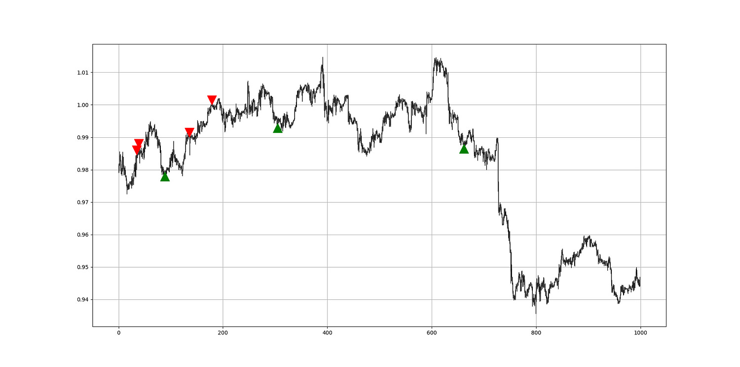
The following Figure shows an example of a signal chart.
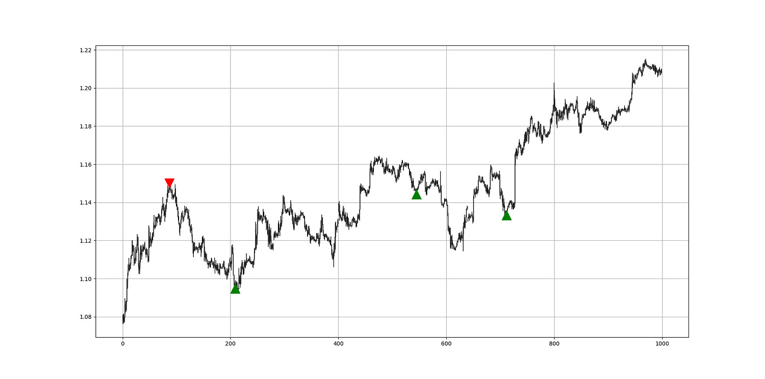
The following Figure shows an example of a signal chart.
Performance Evaluation
If we perform a simple back-test to assess the predictive power of the strategy on GBPUSD and USDCHF, we will find the following results:

The results show positive added value from the strategy and a potential predictive ability. More research is needed into how to optimize the strategy.
If you liked this article, do not hesitate to like and comment, to further the discussion!