The Stochastic Keltner Trading Strategy in Python

Creating and Back-testing a Contrarian Trading Strategy in Python

Dec 09, 2022

This article discusses a trading strategy based on the stochastic oscillator and the Keltner channel, a known volatility indicator. The strategy’s type is contrarian and is best used in ranging markets. The second part of the article will deal with performance evaluation on a selected sample of markets.

Knowledge must be accessible to everyone. This is why, from now on, a purchase of either one of my new books “Contrarian Trading Strategies in Python” or “Trend Following Strategies in Python” comes with free PDF copies of my first three books (Therefore, purchasing one of the new books gets you 4 books in total). The two new books listed above feature a lot of advanced indicators and strategies with a GitHub page. You can use the below link to purchase one of the two books (Please specify which one and make sure to include your e-mail in the note).

Pay Kaabar using PayPal.Me
Go to paypal.me/sofienkaabar and type in the amount. Since it’s PayPal, it’s easy and secure. Don’t have a PayPal…www.paypal.com

The Stochastic Oscillator

The stochastic oscillator is a known bounded technical indicator based on the normalization function. It traps the high, low, and close prices between 0 and 100 so as we get a glance on overstretched markets.

The stochastic oscillator (raw version) is calculated as follows:

Subtract the current close from the lowest low during the last 14 periods. Let’s call this step one.
Subtract the highest high during the last 14 periods from he lowest low during the last 14 periods. Let’s call this step two.
Divide step one by step two and multiply by 100.

The result is the raw version of the stochastic oscillator. The function we can use to code the stochastic oscillator given a numpy OHLC array is as follows:

def stochastic_oscillator(data, 
                             lookback, 
                             high, 
                             low, 
                             close, 
                             position, 
                             slowing = False, 
                             smoothing = False, 
                             slowing_period = 1, 
                             smoothing_period = 1):
            
    data = add_column(data, 1)
        
    for i in range(len(data)):
            
        try:
            
            data[i, position] = (data[i, close] - min(data[i - lookback + 1:i + 1, low])) / (max(data[i - lookback + 1:i + 1, high]) - min(data[i - lookback + 1:i + 1, low]))
            
        except ValueError:
            
            pass
        
    data[:, position] = data[:, position] * 100  
            
    if slowing == True and smoothing == False:
        
        data = ma(data, slowing_period, position, position + 1)
    
    if smoothing == True and slowing == False:
        
        data = ma(data, smoothing_period, position, position + 1)
        
    if smoothing == True and slowing == True:
    
        data = ma(data, slowing_period, position,   position + 1)
        
        data = ma(data, smoothing_period, position + 1, position + 2)        
       
    data = delete_row(data, lookback)

    return data

You need to define the primal function first which are needed to make the function work. They are as follows:

def add_column(data, times):
    
    for i in range(1, times + 1):
    
        new = np.zeros((len(data), 1), dtype = float)
        
        data = np.append(data, new, axis = 1)

    return data

def delete_column(data, index, times):
    
    for i in range(1, times + 1):
    
        data = np.delete(data, index, axis = 1)

    return data

def delete_row(data, number):
    
    data = data[number:, ]
    
    return data

def ma(data, lookback, close, position): 
    
    data = add_column(data, 1)
    
    for i in range(len(data)):
           
            try:
                
                data[i, position] = (data[i - lookback + 1:i + 1, close].mean())
            
            except IndexError:
                
                pass
            
    data = delete_row(data, lookback)
    
    return data

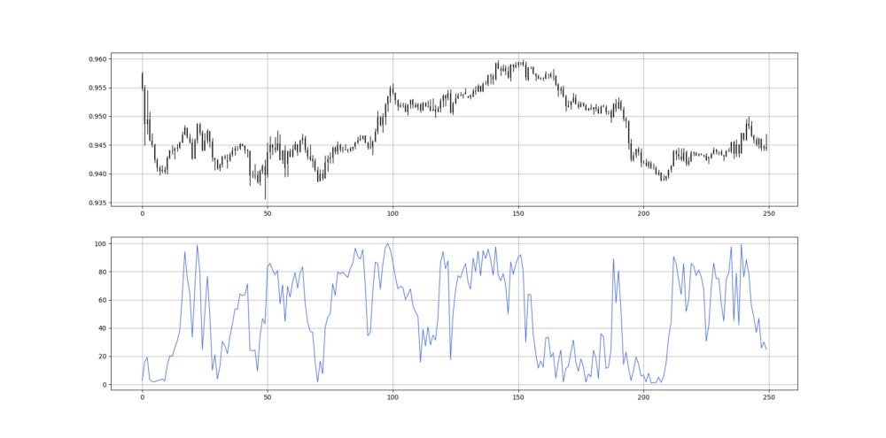
Also, make sure you have an array and not a data frame as the code exclusively works with arrays. The following Figure shows an example of the 14-period stochastic oscillator.

The Keltner Channel

The Keltner channel is a volatility bands indicator which tries to envelop the market price so as to find dynamic support and resistance levels. The steps used to calculate the Keltner channel are as follows:

Calculate an exponential moving average on the close prices.
Calculate an average true range (ATR) using the specified lookback period.
Add step one to step two and multiply by a constant.
Subtract step one from step two and multiply by a constant.

The function we can use to code the Keltner channel given a numpy OHLC array is as follows:

def keltner_channel(data, lookback, multiplier, close, position):
    
    data = add_column(data, 2)
    
    data = ema(data, 2, lookback, close, position)
    
    data = atr(data, lookback, 1, 2, 3, position + 1)
    
    data[:, position + 2] = data[:, position] + (data[:, position + 1] * multiplier)
    data[:, position + 3] = data[:, position] - (data[:, position + 1] * multiplier)

    data = delete_column(data, position, 2)
    data = delete_row(data, lookback)

    return data

Two additional functions must be defined for the above code to work and they are the functions of the Keltner channnel, smoothed moving average, and exponential moving average.

def ema(data, alpha, lookback, close, position):
    
    alpha = alpha / (lookback + 1.0)
    
    beta  = 1 - alpha
    
    data = ma(data, lookback, close, position)

    data[lookback + 1, position] = (data[lookback + 1, close] * alpha) + (data[lookback, position] * beta)

    for i in range(lookback + 2, len(data)):
        
            try:
                
                data[i, position] = (data[i, close] * alpha) + (data[i - 1, position] * beta)
        
            except IndexError:
                
                pass
            
    return data

def smoothed_ma(data, alpha, lookback, close, position):
    
    lookback = (2 * lookback) - 1
    
    alpha = alpha / (lookback + 1.0)
    
    beta  = 1 - alpha
    
    data = ma(data, lookback, close, position)

    data[lookback + 1, position] = (data[lookback + 1, close] * alpha) + (data[lookback, position] * beta)

    for i in range(lookback + 2, len(data)):
        
            try:
                
                data[i, position] = (data[i, close] * alpha) + (data[i - 1, position] * beta)
        
            except IndexError:
                
                pass
            
    return data

def atr(data, lookback, high_column, low_column, close_column, position):
    
    data = add_column(data, 1)
      
    for i in range(len(data)):
        
        try:
            
            data[i, position] = max(data[i, high_column] - data[i, low_column], abs(data[i, high_column] - data[i - 1, close_column]), abs(data[i, low_column]  - data[i - 1, close_column]))
            
        except ValueError:
            
            pass
        
    data[0, position] = 0   
      
    data = smoothed_ma(data, 2, lookback, position, position + 1)

    data = delete_column(data, position, 1)
    
    data = delete_row(data, lookback)
    
    return data

The following Figure shows an example of the 20-period Keltner channel.

Creating the Strategy

The strategy is simple and has the following conditions:

A bullish signal is generated whenever the 14-period stochastic oscillator is lower than 10 while the market has just surpassed the lower Keltner.
A bearish signal is generated whenever the 14-period stochastic oscillator is above 90 while the market has just broken to the downside the upper Keltner.

def signal(data, close_column, stochastic_column, 
           upper_keltner, lower_keltner, buy_column, sell_column):

    data = add_column(data, 5)
    
    for i in range(len(data)):
        
       try:
           
           # Bullish pattern
           if data[i, stochastic_column] < lower_barrier and \
              data[i, close_column] > data[i, lower_keltner] and \
              data[i - 1, close_column] < data[i - 1, lower_keltner]:
                  
                    data[i + 1, buy_column] = 1
                    
           # Bearish pattern
           elif data[i, stochastic_column] > upper_barrier and \
                data[i, close_column] < data[i, upper_keltner] and \
                data[i - 1, close_column] > data[i - 1, upper_keltner]:
                  
                    data[i + 1, sell_column] = -1
                    
       except IndexError:
            
            pass
        
    return data

The following Figure shows an example of a signal chart.

Performance Evaluation

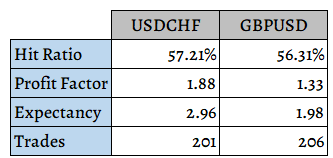
If we perform a simple back-test to assess the predictive power of the strategy on GBPUSD and USDCHF, we will find the following results:

The results show positive added value from the strategy and a potential predictive ability. More research is needed into how to optimize the strategy.

If you want to see how to create all sorts of algorithms yourself, feel free to check out Lumiwealth. From algorithmic trading to blockchain and machine learning, they have hands-on detailed courses that I highly recommend.

Learn Algorithmic Trading with Python Lumiwealth
Learn how to create your own trading algorithms for stocks, options, crypto and more from the experts at Lumiwealth. Click to learn more

Summary

To sum up, what I am trying to do is to simply contribute to the world of objective technical analysis which is promoting more transparent techniques and strategies that need to be back-tested before being implemented. This way, technical analysis will get rid of the bad reputation of being subjective and scientifically unfounded.

I recommend you always follow the the below steps whenever you come across a trading technique or strategy:

Have a critical mindset and get rid of any emotions.
Back-test it using real life simulation and conditions.
If you find potential, try optimizing it and running a forward test.
Always include transaction costs and any slippage simulation in your tests.
Always include risk management and position sizing in your tests.

Finally, even after making sure of the above, stay careful and monitor the strategy because market dynamics may shift and make the strategy unprofitable.

All About Trading!

Discussion about this post