
The Simplest Mean Reversion Trading Strategy
Creating a Very Basic Mean Reversion Strategy in Python


Mean reversion is a type of contrarian trading where the trader expects the price to return to some form of equilibrium which is generally measured by a mean or another central tendency statistic. This article discusses a really simple mean reversion trading strategy.
Quick Introduction to Mean Reversion
Markets generally move in irregular cycles. This means that, when we look at the charts, we tend to see ups, downs, and relatively flat phases. The key to trading and investing is to be able to determine the changes in these phases which are also called market regimes.
Mean reversion can be in the form of a moving average where if the market goes too far from it, it is likely to go back to its area. The following Figure illustrates the example.

But how do we measure ‘too far’? We will try a very simple way based only on the position of the price relative to the moving average.
Getting healthier means changing your lifestyle. Noom Weight helps users lose weight in a sustainable way through behavioral change psychology. It's a no-brainer.

Designing the Strategy
From the last section, we have clear objectives to start designing the strategy:
A long (buy) signal is generated whenever the market goes so far below its moving average that it is likely to revert to the mean higher.
A short (sell) signal is generated whenever the market goes so far above its moving average that it is likely to revert to the mean lower.
The following chart shows signals generated from the strategy described above.
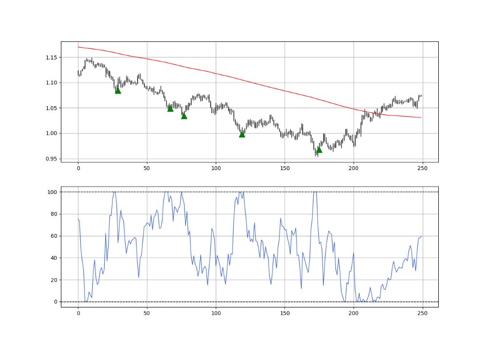
The green arrows represent bullish signals while the red arrows represent bearish signals. To code this normalized distance indicator, we can use the following pseudo code:
# The code assumes you have an OHLC data of historical values imported
# in Python. This has been covered in previous articles

import numpy as np

lookback_ma = 200
lookback_norm = 50

# Defining the primal functions
def add_column(data, times):

    for i in range(1, times + 1):

        new = np.zeros((len(data), 1), dtype = float)

        data = np.append(data, new, axis = 1)

    return data

def delete_column(data, index, times):

    for i in range(1, times + 1):

        data = np.delete(data, index, axis = 1)

    return data

def delete_row(data, number):

    data = data[number:, ]

    return data

# Defining the moving average function
def ma(data, lookback, close, position):

    data = add_column(data, 1)

    for i in range(len(data)):

            try:

                data[i, position] = (data[i - lookback + 1:i + 1, close].mean())

            except IndexError:

                pass

    data = delete_row(data, lookback)

    return data

# Defining the normalization function
def normalized_index(data, lookback, close, position):

    data = add_column(data, 1)

    for i in range(len(data)):

        try:

            data[i, position] = (data[i, close] - min(data[i - lookback + 1:i + 1, close])) / (max(data[i - lookback + 1:i + 1, close]) - min(data[i - lookback + 1:i + 1, close]))

        except ValueError:

            pass

    data[:, position] = data[:, position] * 100

    data = delete_row(data, lookback)

    return data

# Calling a 200-period moving average applied on the close price
my_data = ma(my_data, lookback_ma, 3, 4)

# Adding one extra column for differencing
my_data = add_column(my_data, 10)

# Calculating the absolute distance between the close and the moving average
my_data[:, 5] = abs(my_data[:, 3] - my_data[:, 4])

# Normalizing the distance between 0 and 100 with a period of 50
my_data = normalized_index(my_data, lookback_norm, 5, 6)
Now that we have a 50-period normalized distance between the market and its 200-period moving average, we are ready to code the following trading signals:
A long (buy) signal is generated whenever the normalized index drops from 100 after being equal to 100 while the current close price is less than the close price five periods ago and below the 200-period moving average.
A short (sell) signal is generated whenever the normalized index drops from 100 after being equal to 100 while the current close price is above the close price five periods ago and above the 200-period moving average.
So, this may not be the simplest strategy ever given the conditions, but nevertheless, it is very intuitive and straightforward. The signal function is as follows:
def signal(data, close_column, ma_column, normalized_distance_column, buy_column, sell_column):

    data = add_column(data, 5)

    for i in range(len(data)):

       try:

           # Bullish signal
           if data[i, normalized_distance_column] < 100 and \
              data[i - 1, normalized_distance_column] == 100 and \
              data[i, close_column] < data[i - 5, close_column] and \
              data[i, close_column] < data[i, ma_column]:

                    data[i + 1, buy_column] = 1

           # Bearish signal
           elif data[i, normalized_distance_column] < 100 and \
                data[i - 1, normalized_distance_column] == 100 and \
                data[i, close_column] > data[i - 5, close_column] and \
                data[i, close_column] > data[i, ma_column]:

                    data[i + 1, sell_column] = -1

       except IndexError:

            pass

    return data
The following chart shows another example of signals generated by this strategy.
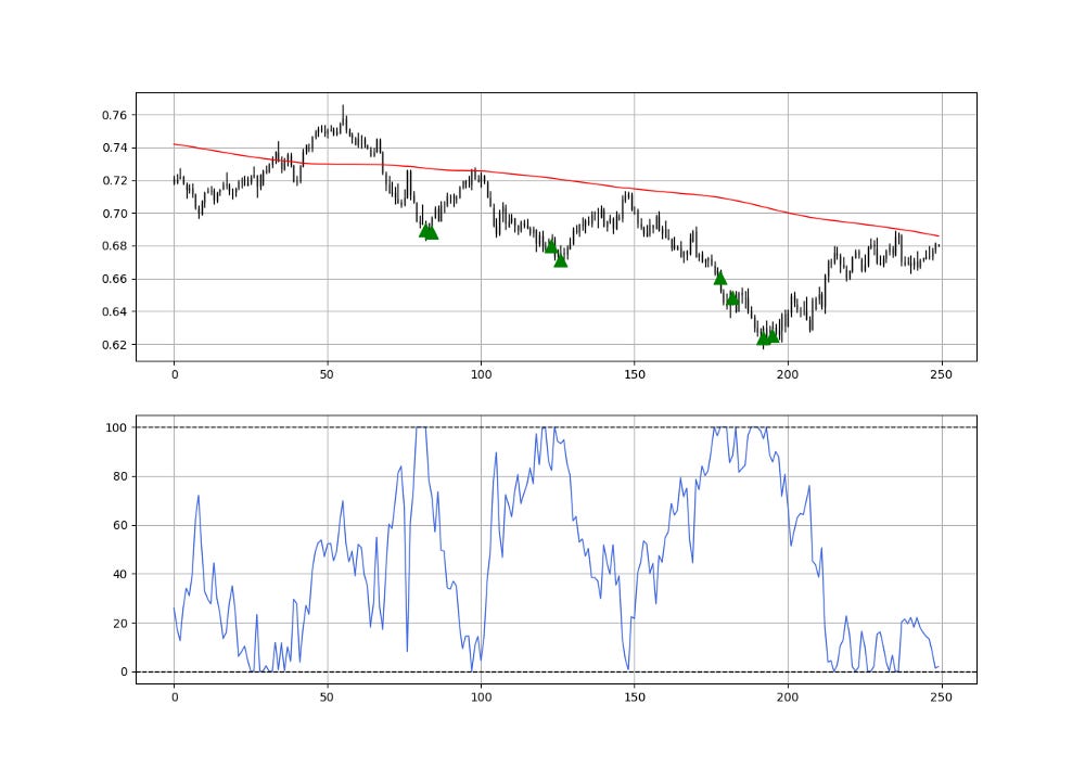
The strategy must be optimized in order to be applied on markets but the idea is to present a mean reversion way of thinking about market analysis.
If you want to see how to create all sorts of algorithms yourself, feel free to check out Lumiwealth. From algorithmic trading to blockchain and machine learning, they have hands-on detailed courses that I highly recommend.
Learn Algorithmic Trading with Python Lumiwealth
Learn how to create your own trading algorithms for stocks, options, crypto and more from the experts at Lumiwealth. Click to learn more
Summary
To sum up, what I am trying to do is to simply contribute to the world of objective technical analysis which is promoting more transparent techniques and strategies that need to be back-tested before being implemented. This way, technical analysis will get rid of the bad reputation of being subjective and scientifically unfounded.
I recommend you always follow the the below steps whenever you come across a trading technique or strategy:
Have a critical mindset and get rid of any emotions.
Back-test it using real life simulation and conditions.
If you find potential, try optimizing it and running a forward test.
Always include transaction costs and any slippage simulation in your tests.
Always include risk management and position sizing in your tests.
Finally, even after making sure of the above, stay careful and monitor the strategy because market dynamics may shift and make the strategy unprofitable.