
The Least Squares Moving Average
Discovering the Merits of the Least Squares Moving Average (LSMA)


Are you a fan of simple moving averages? or maybe exponential moving averages? This article will make you think twice as it presents a lesser-known type of moving average called the least squares moving average.
Moving Averages
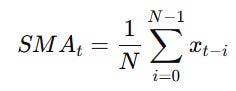
The idea is simple: take the average of a certain number of past data points and slide (or move) this average forward over time. This helps reduce noise and gives a clearer view of the trend. The simple moving average (SMA) is the most basic type. It calculates the arithmetic mean of the last N data points.
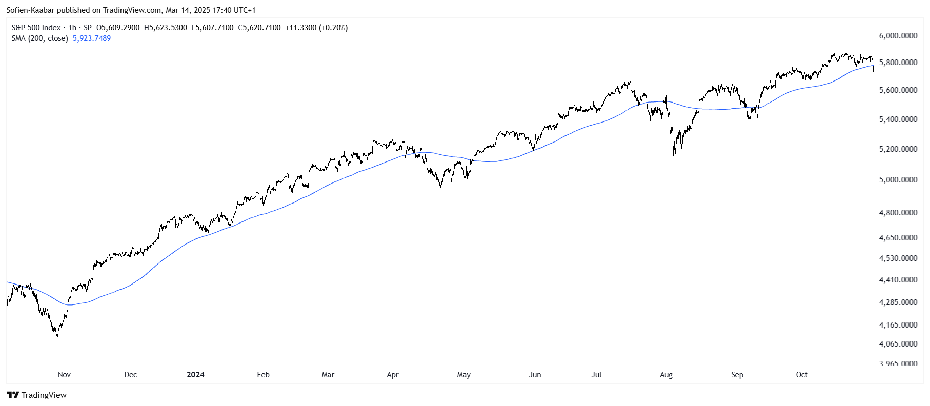
The following chart shows an example of a 200-period SMA.
Moving averages help us detect the trend (is it bullish? bearish? ranging?), but also help us find dynamic support and resistance levels, which are areas from where the prices are expected to react. Take a look at the following chart.
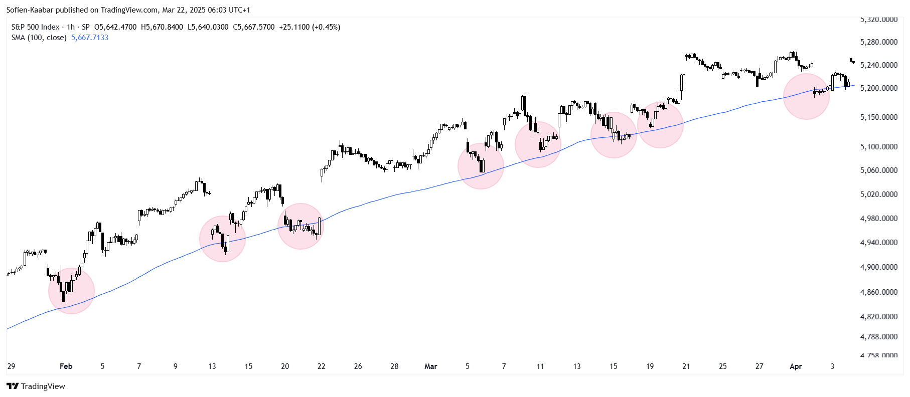
Notice how every time the market goes back to the area around the moving average, it reverses back up. This is the simplest trend following strategy where you re-arm your long (buy) strategy whenever the market corrects. This is in anticipation of a continued bullish trend, and thus you see the corrections as simply better prices to buy.
Least Squares Method
The least squares method is a statistical technique used to find the best-fitting line (or curve) through a set of data points by minimizing the sum of the squares of the vertical distances (errors) between the observed values and the values predicted by the line. Basically, the goal is to find a line:

that minimizes the sum of squared errors:
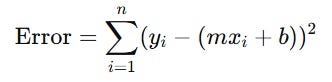
Squaring the errors penalizes large errors more than small ones and ensures all errors are positive (so they don’t cancel each other out). It’s the core idea behind linear regression — modeling the relationship between variables. But in our case, we will be applying this method to a type of moving average.
Least Squares Moving Average
The least squares moving average (LSMA), is a type of moving average that applies the least squares method within a rolling window of data:
For each point in time, take the last n data points.
Fit a linear regression line (via least squares) to those n points.
Use the last value of that regression line as the LSMA for that time point.
Move the window forward by one point and repeat.
Basically, many charting softwares now offer the LSMA, and it seems that it has great potential. Take a look at the following chart featuring a 100-period LSMA on the S&P 500 index.
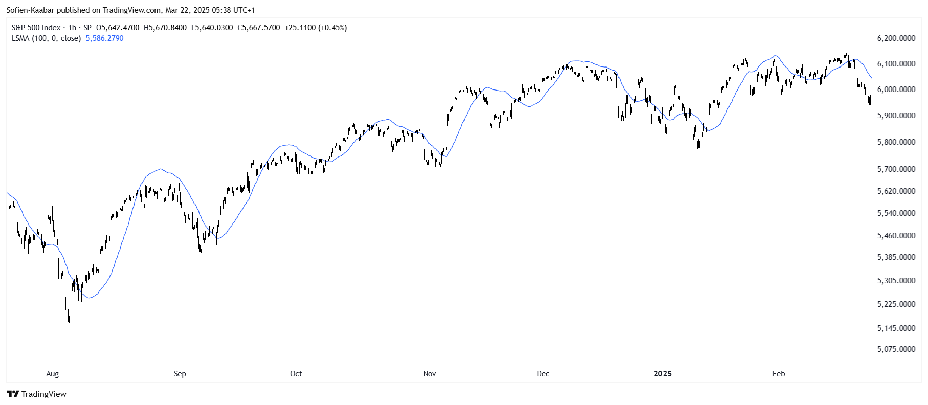
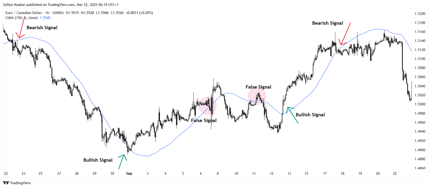
Whenever the market crosses above or under the LSMA, a change in market dynamics occurs. This can be exploited into many types of strategies.
//@version=6
indicator(title = "Least Squares Moving Average", shorttitle="LSMA", overlay=true, timeframe="", timeframe_gaps=true)
length = input(title="Length", defval=25)
offset = input(title="Offset", defval=0)
src = input(close, title="Source")
lsma = ta.linreg(src, length, offset)
plot(lsma, "LSMA")
In comparison to the SMA, the LSMA has the following merits:
It captures linear trends within the lookback period better than SMA.
It reacts faster to price changes due to its regression-based calculation.
It provides a smoother line compared to SMA, especially in trending markets.
Since it uses a linear fit, it can hint at the direction of the trend.
It uses all data in the window but in a statistically optimized way.
Choose wisely!