The LBR Oscillator for Trading
Coding the LBR 3–10 Oscillator in Python
The MACD is a famous oscillator based on moving averages. This article discusses a variation of the MACD called the LBR 3–10.
The Fibonacci Trading Book is finally out! Filled with Fibonacci-based trading methods (tools, indicators, patterns, and strategies), this book will guide you through improving your trading and analysis by incorporating an important technical analysis approach that is Fibonacci [PDF Version available, see end of article).
The Fibonacci Trading Book
Amazon.com: The Fibonacci Trading Book: 9798394344046: Kaabar, Sofien: Booksamzn.to
The MACD Oscillator
The MACD is probably the second most known oscillator after the RSI. One that is heavily followed by traders. It stands for moving average convergence divergence and it is used mainly for divergences and flips. Many people also consider it a trend-following indicator but others use graphical analysis on it to find reversal points, making the MACD a versatile indicator.
As the name suggests, this is your plain simple mean that is used everywhere in statistics and basically any other part in our lives. It is simply the total values of the observations divided by the number of observations. Mathematically speaking, it can be written down as:
The code for the moving average can be written down as the following:
def add_column(data, times):

    for i in range(1, times + 1):

        new = np.zeros((len(data), 1), dtype = float)

        data = np.append(data, new, axis = 1)

    return data
def delete_column(data, index, times):
for i in range(1, times + 1):
data = np.delete(data, index, axis = 1)
return data
def delete_row(data, number):
data = data[number:, ]
return data
def ma(data, lookback, close, position):
data = add_column(data, 1)
for i in range(len(data)):
try:
data[i, position] = (data[i - lookback + 1:i + 1, close].mean())
except IndexError:
pass
#data = delete_row(data, lookback)
return dataThe below states that the moving average function will be called on the array named my_data for a lookback period of 200, on the column indexed at 3 (closing prices in an OHLC array). The moving average values will then be put in the column indexed at 4 which is the one we have added using the adder function.
my_data = ma(my_data, 200, 3, 4)An exponential moving average is a special type that gives more weight to the recent values. To spare you the boring details, here is the code.
def ema(data, alpha, lookback, close, position):

    alpha = alpha / (lookback + 1.0)

    beta  = 1 - alpha

    data = ma(data, lookback, close, position)
    data[lookback + 1, position] = (data[lookback + 1, close] * alpha) + (data[lookback, position] * beta)
    for i in range(lookback + 2, len(data)):

            try:

                data[i, position] = (data[i, close] * alpha) + (data[i - 1, position] * beta)

            except IndexError:

                pass

    return data
How is the MACD calculated? It is the difference between the 26-period exponential moving average applied to the closing price and the 12-period exponential moving average also applied to the closing price. The value found after taking the difference is called the MACD line. The 9-period exponential moving average of that calculation is called the MACD signal. Finally, we take the difference between the MACD line and the MACD signal to find the histogram.
This oscillator is a variation from the MACD created by Linda Bradford Raschke. It uses simple moving averages instead of exponential moving averages. To construct the LBR 3–10, we can follow these steps:
Calculate a 3-period simple moving average.
Calculate a 10-period simple moving average.
Subtract the 3-period moving average from the 10-period moving average. We will call this a MACD line.
Calculate a 16-period simple moving average on the result from the previous step. We will call this a signal line.
Subtract the MACD ine from the signal line. We will call this the histogram line which is the main indicator.
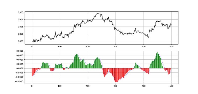
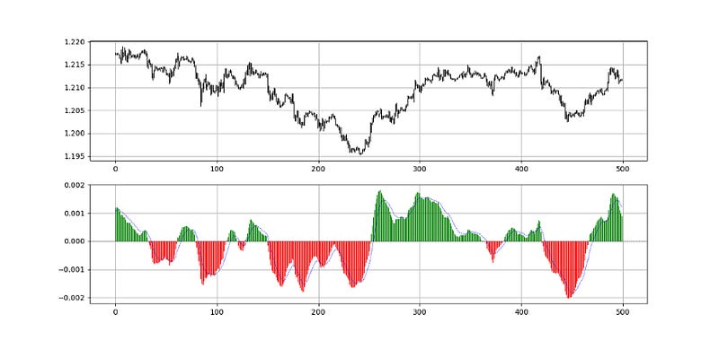
The following Figure shows an example of the LBR 3–10.
def lbr(data, close, long_ema, short_ema, signal_ema, position):

    data = add_column(data, 2)

    data = ma(data, 10,  close, position)
    data = ma(data, 3, close, position + 1)

    data[:, position + 2] = data[:, position + 1] - data[:, position]

    data = ma(data, 16, position + 2, position + 3)

    data[:, position + 4] = data[:, position + 2] - data[:, position + 3]

    data = delete_row(data, 16)
    data = delete_column(data, position, 2)
    data = delete_row(data, signal_ema)

    return data
The following Figure shows an example of the LBR 3–10.
A simple (a bit too simple) strategy on this oscillator is to buy whenever it surpasses zero and to sell whenever it breaks zero. Naturally, with the lag, this strategy is not going to provide good returns but for educational purposes only, it is the default strategy to oscillators that turn around zero.
def signal(data, lbr_column, buy_column, sell_column):

    data = add_column(data, 5)

    for i in range(len(data)):

       try:

           # Bullish pattern
           if data[i, lbr_column] > 0 and data[i - 1, lbr_column] < 0:

                    data[i + 1, buy_column] = 1

           # Bearish pattern
           elif data[i, lbr_column] < 0 and data[i - 1, lbr_column] > 0:

                    data[i + 1, sell_column] = -1

       except IndexError:

            pass

    return data
The PDF link for the Fibonacci Trading Book is the following (make sure to include your e-mail address in the notes part):
Pay Kaabar using PayPal.Me
Go to paypal.me/sofienkaabar and type in the amount. Since it’s PayPal, it’s easy and secure. Don’t have a PayPal…paypal.me


