The Fractal Dimension Index in Trading

Coding the Fractal Dimension Index

Jun 22, 2022

Markets are fractal in nature meaning they possess certain properties such as self-similarity that allows them to be modelled using tools from this field. Of course, this is easier said than done. In this article, we will develop the fractal dimension index in order to analyze the fractality of the market.

I have released a new book called “Contrarian Trading Strategies in Python”. It features a lot of advanced contrarian indicators and strategies with a GitHub page dedicated to the continuously updated code. If you are interested, you could buy the PDF version directly through a PayPal payment of 9.99 EUR.

Please include your email in the note before paying so that you receive it on the right address. Also, once you receive it, make sure to download it through google drive.

Pay Kaabar using PayPal.Me
If you accept cookies, we’ll use them to improve and customize your experience and enable our partners to show you…www.paypal.com

Introduction to Chaos Theory

Chaos theory is a very complex mathematical field that has the job of explaining the effects of very small factors. The butterfly effect comes to mind when thinking of chaos theory. The mentioned effect is the phenomenon where insignificant factors can lead to extreme changes. A chaotic system is an environment that alternates between predictability and randomness, and this is the closest explanation that we have so far for the financial markets.

The efficient market hypothesis fails to thoroughly explain the market dynamics and it is better for now to stick to real trading results and historical performances as a judge for whether markets are predictable or not.

The early experiments with chaos theory occurred with Edward Lorenz, a meteorologist who wanted to simulate weather sequences by incorporating different variables such as temperature and wind speed. Lorenz noticed that whenever he made tiny adjustments in the variables, the final results were extremely different. This was the first proof of the butterfly effect which is one of the pillars of chaos theory.

The assumption in chaos theory with regards to financial markets is that the price is the last thing to change and that the current price is the most important information.

As stated above, Lorenz has proven that chaotic systems are impacted by the slightest changes in their variables. This makes us think about the time where if a certain financial information does not get released or is a bit different, where would the market trade?

Emotions and independent situations all contribute to determining the market price as well. Imagine if a giant hedge fund changed its mind from buying the EUR versus the USD at the last minute and that this information has gone out to the public. Many traders who would have wanted to ride the giant bullish trend along the hedge fund would have eventually changed their minds and this could actually have caused the EURUSD price to go down in value.

The Fractal Dimension Index

The index measures how irregular the time series is and can be considered as a part of the vast chaotic field. When there is a strong trend going on, naturally, the market price is approaching a one-dimensional line and the fractal dimension index approaches 1.0. When the market is choppy and moving sideways, the fractal dimension index approaches 2.0.

**EURUSD in the first panel with the 13-period fractal dimension index in the second panel.**

def fractal_dimension(Data, lookback, high, low, close, where):
    
    Data = adder(Data, 10)
    
    for i in range(len(Data)):
        
        try:
                
            # Calculating N1
            Data[i, where]     = max(Data[i - (2 * lookback):i - lookback, high])
            Data[i, where + 1] = min(Data[i - (2 * lookback):i - lookback, low])
            Data[i, where + 2] = (Data[i, where] - Data[i, where + 1]) / lookback
           
            # Calculating N2
            Data[i, where + 3] = max(Data[i - lookback:i, high])
            Data[i, where + 4] = min(Data[i - lookback:i, low])
            Data[i, where + 5] = (Data[i, where + 3] - Data[i, where + 4]) / lookback
            
            # Calculating N3
            Data[i, where + 6] = max(Data[i, where], Data[i, where + 3])
            Data[i, where + 7] = min(Data[i, where + 1], Data[i, where + 4])
            Data[i, where + 8] = (Data[i, where + 6] - Data[i, where + 7]) / (2 * lookback)
            
            # Calculating the Fractal Dimension Index
            if Data[i, where + 2] > 0 and Data[i, where + 5] > 0 and Data[i, where + 8] > 0:
                
                Data[i, where + 9] = (np.log(Data[i, where + 2] + Data[i, where + 5]) - np.log(Data[i, where + 8])) / np.log(2)
            
        except ValueError:
            pass
        
    # Cleaning
    Data = deleter(Data, where, 9) 
    Data = jump(Data, lookback * 2)
        
    return Data

The way to use the indicator is not straightforward nor is it highly recommended:

Whenever the FDI reaches 1.0, a structural break might occur and a reaction might happen.

The above chart shows reversal signals (non-directional) whenever we use the technique above.

def signal(data, fdi, buy_column):
    
    data = adder(data, 10)
    
    for i in range(len(data)):
        
        try:
            
            if data[i, fdi] < 1 and data[i - 1, fdi] > 1:
                
                data[i + 1, buy_column] = 1
                
        except IndexError:

pass           
        
    return data

Make sure to focus on the concepts and not the code. The most important thing is to comprehend the techniques and strategies. The code is a matter of execution but the idea is something you cook in your head for a while.

Check out my weekly market sentiment report to understand the current positioning and to estimate the future direction of several major markets through complex and simple models working side by side. Find out more about the report through this link:

Coalescence Report 1st May — 8th May 2022
This report covers the weekly market sentiment and positioning and any changes that have occurred which might present…coalescence.substack.com

A Related Calculation — The Hurst Exponent

Financial assets alternate between momentum and mean-reversion as regimes and business cycles change. One way to know whether markets are mean-reverting or trending (thus momentum is prevailing) is to use the Hurst exponent.

The three general types of financial data that can be observed are; trending, mean-reverting, and random walk.

A Trending time series is one that increases or decreases over time. The main characteristic is positive autocorrelation.
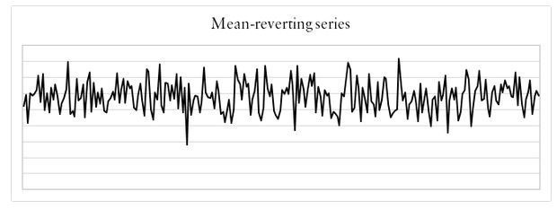
A Mean-reverting time series is one that fluctuates around its long-term equilibrium. The main characteristic is negative autocorrelation.
A Random Walk time series is one that moves randomly over time. The main characteristic is zero autocorrelation.

The random walk theory is the foundation of quantitative finance and is one of the first things a practitioner should understand. Financial data are assumed to follow a random walk and that implies that price movements are random and cannot be forecasted using their past values. Our aim here is to understand which of the three types is the main characteristic of our analyzed data and that question can be answered through the Hurst exponent.

To briefly define this metric, it has been created by British hydrologist, Edwin Hurst during a study on the Nile river in Egypt. We can interpret it in the following three ways:

Whenever H < 0.5, then we can say that our data is mean-reverting.
Whenever H =0.5, then we can say that our data is random.
Whenever H >0.5, then we can say that our data is trending in nature.

If we calculate the Hurst Exponent on real world data, for example the S&P500 index between 2007 and 2019, we find that it is around 0.43. Does this mean that the index is mean-reverting?

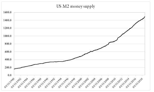
Not necessarily, the calculated value is from the 2007–2019 period and has a range of 30 values which may not capture the whole story. The true value should lie between 0.49 and 0.51 which is closer to a random walk with a pinch of determinism. We cannot negate the possibility that the S&P500 follows no specific pattern whatsoever and although we know that it does from time to time (mostly trending), we merely want to learn how to use the Hurst exponent for quick statistical tests granted we use quality data and optimal parameters such as taking relevant time periods. Another real example is the US M2 money supply. Naturally, it is always upwards sloping.

It is apparent that it is trending overtime, but what does the exponent say? According to the results shown, the Hurst exponent is around 0.744 which is an indication of a highly trending series. Mathematically speaking, the Hurst exponent revolves around the idea of using the variance of a log price series to determine the diffusion. What the function does is compare the diffusion of a time series to that of a geometric Brownian motion, in other words, if the data possesses autocorrelation then the below relationship will not hold and can be modified to include a value of 2H, which is actually the Hurst exponent:

If H = 0.5, then the equation would reduce to the below:

That is the rate of diffusion of a geometric Brownian motion. Tau (𝛕) denotes time and it is equal to the variance at a longer time horizon. The geometric Brownian motion dictates that the variance is equal to the time horizon when it is large enough. It becomes clear now why we say that when the Hurst exponent equals 0.5, we have a random time series. To calculate a rolling measure of the Hurst Exponent, we need to first install the library:

pip install hurst

Next, we can create the function as below:

from hurst import compute_Hcdef hurst(Data, lookback, what, where):

for i in range(len(Data)):
        try:
            new = Data[i - lookback:i, what]
            
            Data[i, where] = compute_Hc(Data[i - lookback:i + 1, what])[0]
        except ValueError:
            pass
        
    return Data

# Using the Function
my_data = hurst(my_data, 100, 3, 4)

Whenever the market starts to trend, its Hurst Exponent starts to rise due to persistency until markets start to consolidate which is when the Hurst starts dropping. The idea of detecting tops in the Hurst to detect market turning points seems reasonable but in practice, it is not very useful as the Hurst does not really follow a clear stationary pattern. Yesterday’s 0.60 barrier is today’s meaningless level.

Summary

To sum up, what I am trying to do is to simply contribute to the world of objective technical analysis which is promoting more transparent techniques and strategies that need to be back-tested before being implemented. This way, technical analysis will get rid of the bad reputation of being subjective and scientifically unfounded.

I recommend you always follow the the below steps whenever you come across a trading technique or strategy:

Have a critical mindset and get rid of any emotions.
Back-test it using real life simulation and conditions.
If you find potential, try optimizing it and running a forward test.
Always include transaction costs and any slippage simulation in your tests.
Always include risk management and position sizing in your tests.

Finally, even after making sure of the above, stay careful and monitor the strategy because market dynamics may shift and make the strategy unprofitable.

All About Trading!

Discussion about this post