The Equilibrium Indicator

Coding and Trading the Reversion to Equilibrium in Python

Markets swing between extremes and move in cyclical phases. Sometimes, they are a bit overbought due to a superior optimistic feeling and other times they are oversold due to looming fear. The self-similarity and fractal natures of the financial markets tell us that this goes for all the time frames. In this article, we will see how to profit from fading extreme moves using the Equilibrium method.

I have just published a new book after the success of New Technical Indicators in Python. It features a more complete description and addition of complex trading strategies with a Github page dedicated to the continuously updated code. If you feel that this interests you, feel free to visit the below link, or if you prefer to buy the PDF version, you could contact me on Linkedin.

The Book of Trading Strategies
Amazon.com: The Book of Trading Strategies: 9798532885707: Kaabar, Sofien: Bookswww.amazon.com

---

The Concept of Moving Averages

Moving averages help us confirm and ride the trend. They are the most known technical indicator and this is because of their simplicity and their proven track record of adding value to the analyses. We can use them to find support and resistance levels, stops and targets, and to understand the underlying trend. This versatility makes them an indispensable tool in our trading arsenal.

EURUSD hourly values with the 200-period simple moving average.

As the name suggests, this is your plain simple mean that is used everywhere in statistics and basically any other part in our lives. It is simply the total values of the observations divided by the number of observations. Mathematically speaking, it can be written down as:

We can see that the moving average is providing decent dynamic support and resistance levels from where we can place our orders in case the market goes down there.

The code for the moving average can be written down as the following:

def ma(Data, lookback, what, where):
    
  for i in range(len(Data)):
      try:
        Data[i, where] = (Data[i - lookback + 1:i + 1, what].mean())
        
            except IndexError:
                pass
    return Data

To use it, we need to have an OHLC data array with an extra empty column. This can be done by using the following code:

# Defining the function that adds a certain number of columns
def adder(Data, times):
    
    for i in range(1, times + 1):
    
        z = np.zeros((len(Data), 1), dtype = float)
        Data = np.append(Data, z, axis = 1)

    return Data

# Adding 1 extra column
my_data = adder(my_data, 1)

# Calling the moving average function
my_data = ma(my_data, 200, 3, 4)

The above states that the moving average function will be called on the array named my_data for a lookback period of 200, on the column indexed at 3 (closing prices in an OHLC array). The moving average values will then be put in the column indexed at 4 which is the one we have added using the adder function.

USDCHF hourly values with the 200-period simple moving average.

The Equilibrium Indicator

The state of Equilibrium can be measured in many complex ways ranging from advanced mathematics to complex computations, but the way I see it is, why complicate things? We can create a very simple proxy to measure the market’s position relative to its implied Equilibrium. By implied, we mean that it can be an average that the market often reverts to. This is usually a short-term moving average where the price frequently closes above and below it.

This means that this short-term moving average is not like the ones we use to find dynamic support and resistance levels, but one that can be used to tell us that the market is likely to go towards its direction.

We will measure Equilibrium as being the exponentially smoothed average of the distance between the market price and its moving average.

This means that we will follow the below steps:

• Calculate a simple 5-period moving average of the market price.

• Subtract the current market price from its moving average.

• Calculate a 5-period exponential moving average on the subtracted values.

The result is the 5-period Equilibrium Indicator that we will use to generate mean-reverting signals.

EURUSD in the first panel with the 5-period Equilibrium Indicator.

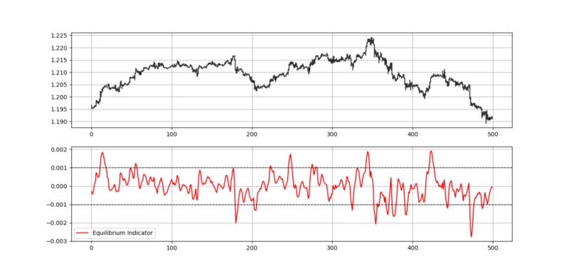
The above plot shows an example on the EURUSD hourly data plotted with the Equilibrium Indicator in blue. The full code can be find below:

def ema(Data, alpha, lookback, what, where):
    
    # alpha is the smoothing factor
    # window is the lookback period
    # what is the column that needs to have its average calculated
    # where is where to put the exponential moving average
    
    alpha = alpha / (lookback + 1.0)
    beta  = 1 - alpha
    
    # First value is a simple SMA
    Data = ma(Data, lookback, what, where)
    
    # Calculating first EMA
    Data[lookback + 1, where] = (Data[lookback + 1, what] * alpha) + (Data[lookback, where] * beta)

    # Calculating the rest of EMA
    for i in range(lookback + 2, len(Data)):
            try:
                Data[i, where] = (Data[i, what] * alpha) + (Data[i - 1, where] * beta)
        
            except IndexError:
                pass
    return Data

def deleter(Data, index, times):
    
    for i in range(1, times + 1):
    
        Data = np.delete(Data, index, axis = 1)

return Data
   
def jump(Data, jump):
    
    Data = Data[jump:, ]
    
    return Data

def equilibrium(Data, lookback, close, where):
    
    # Calculating the moving average
    Data = ma(Data, lookback, close, where)
    Data = jump(Data, lookback)
    
    # Calculating the distance from the moving average
    Data[:, where + 1] = Data[:, close] - Data[:, where]
    
    # Calculating the Exponential Moving Average of the Equilibrium
    Data = ema(Data, 2, lookback, where + 1, where + 2)
    Data = jump(Data, lookback)
    Data = deleter(Data, where, 2)
    
    return Data

# Using the function
my_data = equilibrium(Data, 5, 3, 4)

USDCHF in the first panel with the 5-period Equilibrium Indicator.