
What period should we put on the relative strength index? This question is subjective and is personal to every analyst and trader. One solution to this dilemma is to try to automate the process of choosing the lookback period at every time step. In this article, we will see how to create a dynamically adjusted relative strength index.
I have just released a new book after the success of the previous book. It features advanced trend following indicators and strategies with a GitHub page dedicated to the continuously updated code. Also, this book features the original colors after having optimized for printing costs. If you feel that this interests you, feel free to visit the below Amazon link, or if you prefer to buy the PDF version, you could contact me on LinkedIn.
The Relative Strength Index
First introduced by J. Welles Wilder Jr., the RSI is one of the most popular and versatile technical indicators. Mainly used as a contrarian indicator where extreme values signal a reaction that can be exploited. Typically, we use the following steps to calculate the default RSI:
Calculate the change in the closing prices from the previous ones.
Separate the positive net changes from the negative net changes.
Calculate a smoothed moving average on the positive net changes and on the absolute values of the negative net changes.
Divide the smoothed positive changes by the smoothed negative changes. We will refer to this calculation as the Relative Strength — RS.
Apply the normalization formula shown below for every time step to get the RSI.
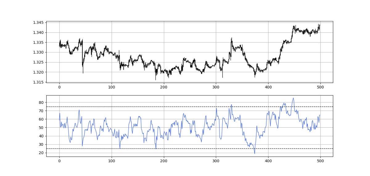
The above chart shows the hourly values of the GBPUSD in black with the 13-period RSI. We can generally note that the RSI tends to bounce close to 25 while it tends to pause around 75. To code the RSI in Python, we need an OHLC array composed of four columns that cover open, high, low, and close prices.
def adder(data, times):

    for i in range(1, times + 1):

        new = np.zeros((len(data), 1), dtype = float)

        data = np.append(data, new, axis = 1)
return datadef deleter(data, index, times):
for i in range(1, times + 1):
data = np.delete(data, index, axis = 1) return data
def jump(data, jump):
data = data[jump:, ]
return datadef ma(data, lookback, close, where):
data = adder(data, 1)
for i in range(len(data)):
try:
data[i, where] = (data[i - lookback + 1:i + 1, close].mean())
except IndexError:
pass
data = jump(data, lookback)
return datadef ema(data, alpha, lookback, what, where):
alpha = alpha / (lookback + 1.0)
beta = 1 - alpha
data = ma(data, lookback, what, where)data[lookback + 1, where] = (data[lookback + 1, what] * alpha) + (data[lookback, where] * beta) for i in range(lookback + 2, len(data)):
try:
data[i, where] = (data[i, what] * alpha) + (data[i - 1, where] * beta)
except IndexError:
pass
return datadef rsi(data, lookback, close, where):
data = adder(data, 5)
for i in range(len(data)):
data[i, where] = data[i, close] - data[i - 1, close]
for i in range(len(data)):
if data[i, where] > 0:
data[i, where + 1] = data[i, where]
elif data[i, where] < 0:
data[i, where + 2] = abs(data[i, where])
lookback = (lookback * 2) - 1 # From exponential to smoothed
data = ema(data, 2, lookback, where + 1, where + 3)
data = ema(data, 2, lookback, where + 2, where + 4) data[:, where + 5] = data[:, where + 3] / data[:, where + 4]
data[:, where + 6] = (100 - (100 / (1 + data[:, where + 5]))) data = deleter(data, where, 6)
data = jump(data, lookback) return dataThe Relative Volatility Index
Our first step into calculating the dynamic relative strength index is to calculate the relative volatility index. Volatility is the magnitude of fluctuations of a variable around its mean value. In time series, a volatile data is one that moves swiftly from one level to another and is generally away from its mean while a stable or low-volatility data is one that looks closer to its moving average (mean).

There are many ways to measure volatility such as the average true range, the mean absolute deviation, and the standard deviation. We will use standard deviation to create the relative volatility index.
The most basic type of volatility is the standard deviation. It is one of the pillars of descriptive statistics and an important element in some technical indicators such as the famous Bollinger bands. But first let us define what variance is before we find the standard deviation.
Variance is the squared deviations from the mean (a dispersion measure), we take the square deviations so as to force the distance from the mean to be non-negative, finally we take the square root to make the measure have the same units as the mean, in a way we are comparing apples to apples (mean to standard deviation standard deviation). Variance is calculated through this formula:

Following what we have said, standard deviation is therefore:

def volatility(Data, lookback, what, where):

  for i in range(len(Data)):
try: Data[i, where] = (Data[i - lookback + 1:i + 1, what].std()) except IndexError: pass
return DataThe exciting job now is to turn the historical volatility otherwise known as the historical standard deviation into an understandable indicator that resembles the relative strength index. The below plot shows the relative volatility index which is simply the RSI applied to 10-period standard deviation of the closing prices.

If you are also interested by more technical indicators and strategies, then my book might interest you:
Creating the Dynamic Relative Strength Index
The idea of the dynamic relative strength index is to select the lookback period based on the recent volatility following this intuition:
Whenever the volatility is high according to the current RVI, we need to bias the lookback period on the RSI downwards to account more for the recent values.
Whenever the volatility is low according to the current RVI, we need to bias the lookback period on the RSI upwards to account less for the recent values.
Therefore, the two main components of the dynamic relative strength index are:
The relative volatility index.
The relative strength index.
How are we going to calculate this and how does it use volatility? It is a very simple concept, let us take a look at the below code:
lookback = 10def dynamic_relative_strength_index(data, lookback, close, where):
# Calculating the Relative Volatility Index
data = relative_volatility_index(data, lookback, close, where)
# Adding a column
data = adder(data, 1)
# Calculating the Lookback Periods on the Dynamic Relative Strength Index
for i in range(len(data)):
if data[i, where] >= 0 and data[i, where] <= 10 :
data[i, where + 1] = 90
if data[i, where] > 10 and data[i, where] <= 20 :
data[i, where + 1] = 80
if data[i, where] > 20 and data[i, where] <= 30 :
data[i, where + 1] = 70
if data[i, where] > 30 and data[i, where] <= 40 :
data[i, where + 1] = 60
if data[i, where] > 40 and data[i, where] <= 50 :
data[i, where + 1] = 50
if data[i, where] > 50 and data[i, where] <= 60 :
data[i, where + 1] = 40
if data[i, where] > 60 and data[i, where] <= 70 :
data[i, where + 1] = 30
if data[i, where] > 70 and data[i, where] <= 80 :
data[i, where + 1] = 20
if data[i, where] > 80 and data[i, where] <= 90 :
data[i, where + 1] = 10
if data[i, where] > 90 and data[i, where] <= 100 :
data[i, where + 1] = 5
# Calculating the Relative Strength Index
data = rsi(data, 5, close, where + 2)
data = rsi(data, 10, close, where + 3)
data = rsi(data, 20, close, where + 4)
data = rsi(data, 30, close, where + 5)
data = rsi(data, 40, close, where + 6)
data = rsi(data, 50, close, where + 7)
data = rsi(data, 60, close, where + 8)
data = rsi(data, 70, close, where + 9)
data = rsi(data, 80, close, where + 10)
data = rsi(data, 90, close, where + 11)
# Adding a column
data = adder(data, 1)
# Dynamic Relative Strength Index
for i in range(len(data)):
if data[i, where + 1] == 5:
data[i, where + 12] = data[i, where + 2]
if data[i, where + 1] == 10:
data[i, where + 12] = data[i, where + 3]
if data[i, where + 1] == 20:
data[i, where + 12] = data[i, where + 4]
if data[i, where + 1] == 30:
data[i, where + 12] = data[i, where + 5]
if data[i, where + 1] == 40:
data[i, where + 12] = data[i, where + 6]
if data[i, where + 1] == 50:
data[i, where + 12] = data[i, where + 7]
if data[i, where + 1] == 60:
data[i, where + 12] = data[i, where + 8]
if data[i, where + 1] == 70:
data[i, where + 12] = data[i, where + 9]
if data[i, where + 1] == 80:
data[i, where + 12] = data[i, where + 10]
if data[i, where + 1] == 90:
data[i, where + 12] = data[i, where + 11]
# Cleaning
data = deleter(data, where, 12)
return dataWhat the above code simply does is calculate the 10-period relative volatility index, then calculates an array of RSI’s on the market price using the following lookback periods {5, 10, 20, 30, 40, 50, 60, 70, 80, 90}. Then the code will loop around the data and segment the relative volatility index into 10 parts with each part assigned a period. For example:
If the RVI is showing a reading of 8, then it falls into the first part. With such low volatility, the lookback calculated on the RSI is 90. This is to account for the low current volatility.
If the RVI is showing a reading of 85, then it falls into the ninth part. With such high volatility, the lookback calculated on the RSI is 10. This is to account for the high current volatility.

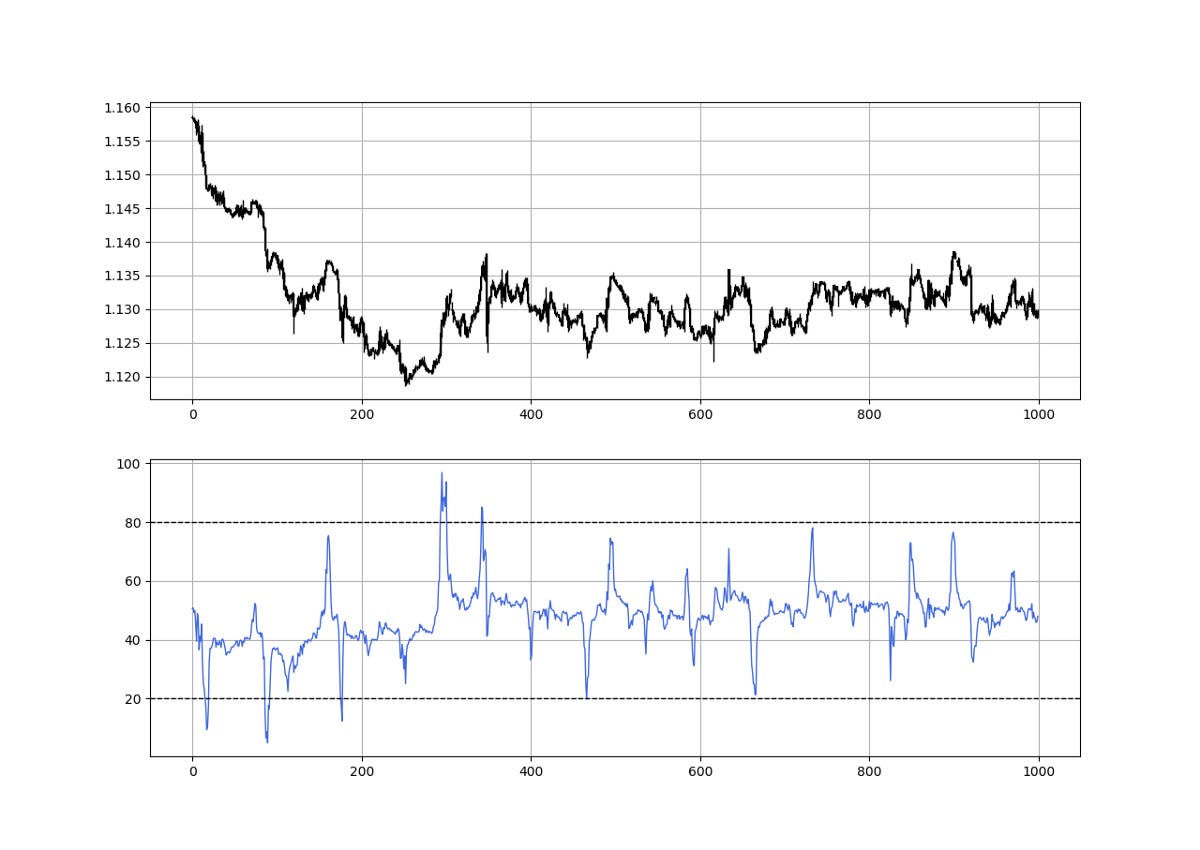
The dynamic relative strength index witnesses from time to time spikes and this due to the change in volatility. It takes into account the current market properties and is therefore better at detecting short-term and long-term opportunities and signals. Unlike the normal RSI, the dynamic RSI, when around 50, does not mean we are far from a signal due to the fact that it can spike at any time.
Remember to always do your back-tests. You should always believe that other people are wrong. My indicators and style of trading may work for me but maybe not for you.
I am a firm believer of not spoon-feeding. I have learnt by doing and not by copying. You should get the idea, the function, the intuition, the conditions of the strategy, and then elaborate (an even better) one yourself so that you back-test and improve it before deciding to take it live or to eliminate it. My choice of not providing specific Back-testing results should lead the reader to explore more herself the strategy and work on it more.
One Last Word
I have recently started an NFT collection that aims to support different humanitarian and medical causes. The Society of Light is a set of limited collectibles which will help make the world slightly better as each sale will see a percentage of it sent directly to the charity attributed to the avatar. As I always say, nothing better than a bullet list to outline the benefits of buying these NFT’s:
High-potential gain: By concentrating the remaining sales proceedings on marketing and promoting The Society of Light, I am aiming to maximize their value as much as possible in the secondary market. Remember that trading in the secondary market also means that a portion of royalties will be donated to the same charity.
Art collection and portfolio diversification: Having a collection of avatars that symbolize good deeds is truly satisfying. Investing does not need to only have selfish needs even though there is nothing wrong with investing to make money. But what about investing to make money, help others, and collect art?
Donating to your preferred cause(s): This is a flexible way of allocating different funds to your charities.
A free copy of my book in PDF: Any buyer of any NFT will receive a free copy of my latest book shown in the link of the article.