The Bollinger Bands Width Indicator

Coding & Presenting the Bollinger Bands Width Indicator in Python

Aug 29, 2022

We can transform Bollinger bands so that we measure their width, thus helping us understanding whether Bollinger bands-based strategies will work better or not. This article presents the details of the Bollinger bands width indicator.

I have released a new book called “Contrarian Trading Strategies in Python”. It features a lot of advanced contrarian indicators and strategies with a GitHub page dedicated to the continuously updated code. If you are interested, you could buy the PDF version directly through a PayPal payment of 9.99 EUR.

Please include your email in the note before paying so that you receive it on the right address. Also, once you receive it, make sure to download it through google drive.

Pay Kaabar using PayPal.Me
If you accept cookies, we’ll use them to improve and customize your experience and enable our partners to show you…www.paypal.com

Bollinger Bands

What are the Bollinger bands? When prices move, we can calculate a moving average (mean) around them so that we better understand their position regarding their mean. By doing this we can also calculate where do they stand statistically. But first we need to understand the concept of the normal distribution curve which is the essence of statistics and the foundation of statistical theory.

**An example of the Normal Distribution Curve.**

The above curve shows the number of values within a number of standard deviations. For example, the area shaded in red represents around 1.33x of standard deviations away from the mean of zero. We know that if data is normally distributed then:

About 68% of the data falls within 1 standard deviation of the mean.
About 95% of the data falls within 2 standard deviations of the mean.
About 99% of the data falls within 3 standard deviations of the mean.

Presumably, this can be used to approximate the way to use financial returns data, but studies show that financial data is not normally distributed but at the moment we can assume it is so that we can use such indicators. The issue with the method does not hinder much its usefulness.

Hence, the Bollinger bands are simple a combination of a moving average that follows prices and a moving standard deviation(s) band that moves alongside the price and the moving average.

To calculate the two Bands, we use the following relatively simple formulas:

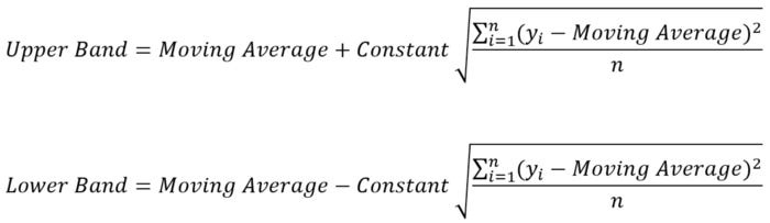
With the constant being the number of standard deviations that we choose to envelop prices with. By default, the indicator calculates a 20-period simple moving average and two standard deviations away from the price, then plots them together to get a better understanding of any statistical extremes. This means that on any time, we can calculate the mean and standard deviations of the last 20 observations we have and then multiply the standard deviation by the constant. Finally, we can add and subtract it from the mean to find the upper and lower band.

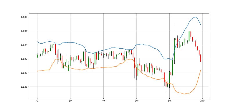
Clearly, the below chart seems easy to understand. Every time the price reaches one of the bands, a contrarian position is most suited and this is evidenced by the reactions we tend to see when prices hit these extremes. So, whenever the EURUSD reaches the upper band, we can say that statistically, it should consolidate and when it reaches the lower band, we can say that statistically, it should bounce.

**EURUSD with the 20-period Bollinger bands.**

To create the Bollinger bands in Python, we need to define the moving average function, the standard deviation function, and then the Bollinger bands function which will use the former two functions. Note that this should be used on OHLC data array with a few columns to spare.

def adder(data, times):
    
    for i in range(1, times + 1):
    
        new = np.zeros((len(data), 1), dtype = float)
        
        data = np.append(data, new, axis = 1)

return data

def deleter(data, index, times):
    
    for i in range(1, times + 1):
    
        data = np.delete(data, index, axis = 1)

return data
   
def jump(data, jump):
    
    data = data[jump:, ]
    
    return data

def ma(data, lookback, close, where): 
    
    data = adder(data, 1)
    
    for i in range(len(data)):
           
            try:
                
                data[i, where] = (data[i - lookback + 1:i + 1, close].mean())
            
            except IndexError:
                
                pass
            
    data = jump(data, lookback)
    
    return data

def volatility(Data, lookback, what, where):
    
    for i in range(len(Data)):
      try:
        Data[i, where] = (Data[i - lookback + 1:i + 1, what].std())
    
        except IndexError:
            pass
        
    return Data

def bollinger_bands(data, boll_lookback, standard_distance, what, where):
       
    data = adder(data, 2)
    
    data = ma(data, boll_lookback, what, where)    data = volatility(data, boll_lookback, what, where + 1)
    
    data[:, where + 2] = data[:, where] + (standard_distance * data[:, where + 1])

data[:, where + 3] = data[:, where] - (standard_distance * data[:, where + 1])
    
    data = jump(data, boll_lookback)
    
    data = deleter(data, where + 1, 1)
        
    return data

Bollinger Bands Width

The width of this indicator measure the relative distance between the bands and the moving average used to create them.

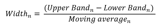
We tend to see the width go up whenever there is severe trending that causes the distance between the two bands to grow.

def bollinger_width(data, ma_col, upper_boll, lower_boll, where):
    
    data = adder(data, 1)
    
    for i in range(len(data)):
        
        data[i, where] = (data[i, upper_boll] - data[i, lower_boll]) / data[i, ma_col]
        
    return data

Using the Bollinger Bands Width

Using the Bollinger bands width is simple. Whenever the Bollinger bands widen, the width indicator increases until they start converging. The only known method of using the width is regime alternation. This signifies that whenever the width is relatively high, the current trend may end soon and whenever it is relatively low, there might be a breakout either upwards or downwards.

Summary

To sum up, what I am trying to do is to simply contribute to the world of objective technical analysis which is promoting more transparent techniques and strategies that need to be back-tested before being implemented. This way, technical analysis will get rid of the bad reputation of being subjective and scientifically unfounded.

I recommend you always follow the the below steps whenever you come across a trading technique or strategy:

Have a critical mindset and get rid of any emotions.
Back-test it using real life simulation and conditions.
If you find potential, try optimizing it and running a forward test.
Always include transaction costs and any slippage simulation in your tests.
Always include risk management and position sizing in your tests.

Finally, even after making sure of the above, stay careful and monitor the strategy because market dynamics may shift and make the strategy unprofitable.

For the paperback link of the book, you may use the following link:

Contrarian Trading Strategies in Python
Amazon.com: Contrarian Trading Strategies in Python: 9798434008075: Kaabar, Sofien: Bookswww.amazon.co

All About Trading!

Discussion about this post