

Imagine a drunk person walking home at night. Each step could go forward or backward — unpredictable, chaotic, driven by chance. Now ask: Can we predict where they’ll end up after 100 steps?
Not exactly. But surprisingly, we can predict the average distance they’ll be from the start, and how that uncertainty grows with time.
That’s the strange beauty of randomness — it looks chaotic up close, yet reveals structure when you step back. Stochastic calculus is the mathematics that makes sense of that structure. It’s calculus for systems driven by noise.
From Random Walks to Brownian Motion
Let’s start small — literally. A random walk is just a sequence of random steps:

where each ϵ is +1 or –1 with equal probability. If you repeat this process, your path will wiggle around unpredictably. But over many runs, a clear pattern emerges: the expected position stays near zero, and the spread of positions grows steadily.
If you make the steps smaller and take them more frequently, the motion becomes continuous. In the limit, we get Brownian motion (also called a Wiener process):
a continuous, nowhere-differentiable path that models pure randomness.
Do you want to master Deep Learning techniques tailored for time series, trading, and market analysis🔥? My book breaks it all down from basic machine learning to complex multi-period LSTM forecasting while going through concepts such as fractional differentiation and forecasting thresholds. Get your copy here 📖!
Python Demo: Simulating a Random Walk and Brownian Motion
Here’s a simple simulation to see this in action:
import numpy as np
import matplotlib.pyplot as plt

# Parameters
N = 1000        # number of steps
dt = 0.01       # time step
t = np.linspace(0, N*dt, N)

# Simulate multiple Brownian motion paths
num_paths = 10
paths = np.zeros((num_paths, N))

for i in range(num_paths):
    dW = np.random.randn(N) * np.sqrt(dt)
    W = np.cumsum(dW)
    paths[i] = W

# Plot the paths
plt.figure(figsize=(10, 5))
for i in range(num_paths):
    plt.plot(t, paths[i], lw=1)
plt.title(”Simulated Brownian Motion Paths”)
plt.xlabel(”Time”)
plt.ylabel(”Position”)
plt.grid(True)
plt.show()
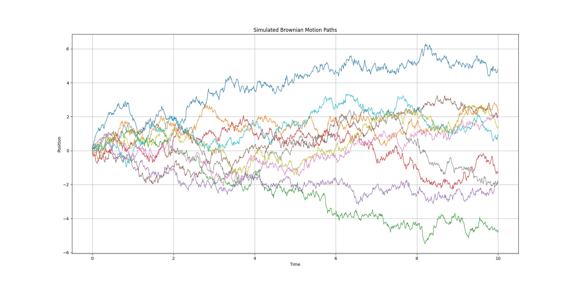
Each line on the plot is one possible “drunkard’s journey.” No two are alike, but all share the same structure — wandering around zero, spreading out over time.
There’s a catch. A Brownian path is so irregular it’s nowhere differentiable — the slope changes infinitely fast. Traditional calculus fails here. That’s where stochastic calculus comes in. It rewrites the rules of differentiation and integration to handle randomness.
In this new world:

That tiny equation is the key to the entire theory. It captures the idea that the square of a random fluctuation grows linearly with time, the seed of all diffusion, noise, and uncertainty.
You can think of it as calculus that works on roads made of static and vibration.
Let’s make randomness measurable.
For Brownian motion Wt:
E[Wt] = 0 → average position is zero.
Var(Wt) = t → uncertainty grows linearly with time.
Even chaos has rules. We can check these facts numerically:
num_paths = 5000
N = 1000
dt = 0.01
t = np.linspace(0, N*dt, N)

# Simulate many paths
paths = np.cumsum(np.random.randn(num_paths, N) * np.sqrt(dt), axis=1)

# Compute mean and variance across paths
mean = paths.mean(axis=0)
var = paths.var(axis=0)

# Plot
plt.figure(figsize=(10, 5))
plt.subplot(1, 2, 1)
plt.plot(t, mean)
plt.title(”Mean of Brownian Motion (≈ 0)”)
plt.xlabel(”Time”)
plt.ylabel(”Mean”)

plt.subplot(1, 2, 2)
plt.plot(t, var)
plt.title(”Variance of Brownian Motion (≈ t)”)
plt.xlabel(”Time”)
plt.ylabel(”Variance”)

plt.tight_layout()
plt.show()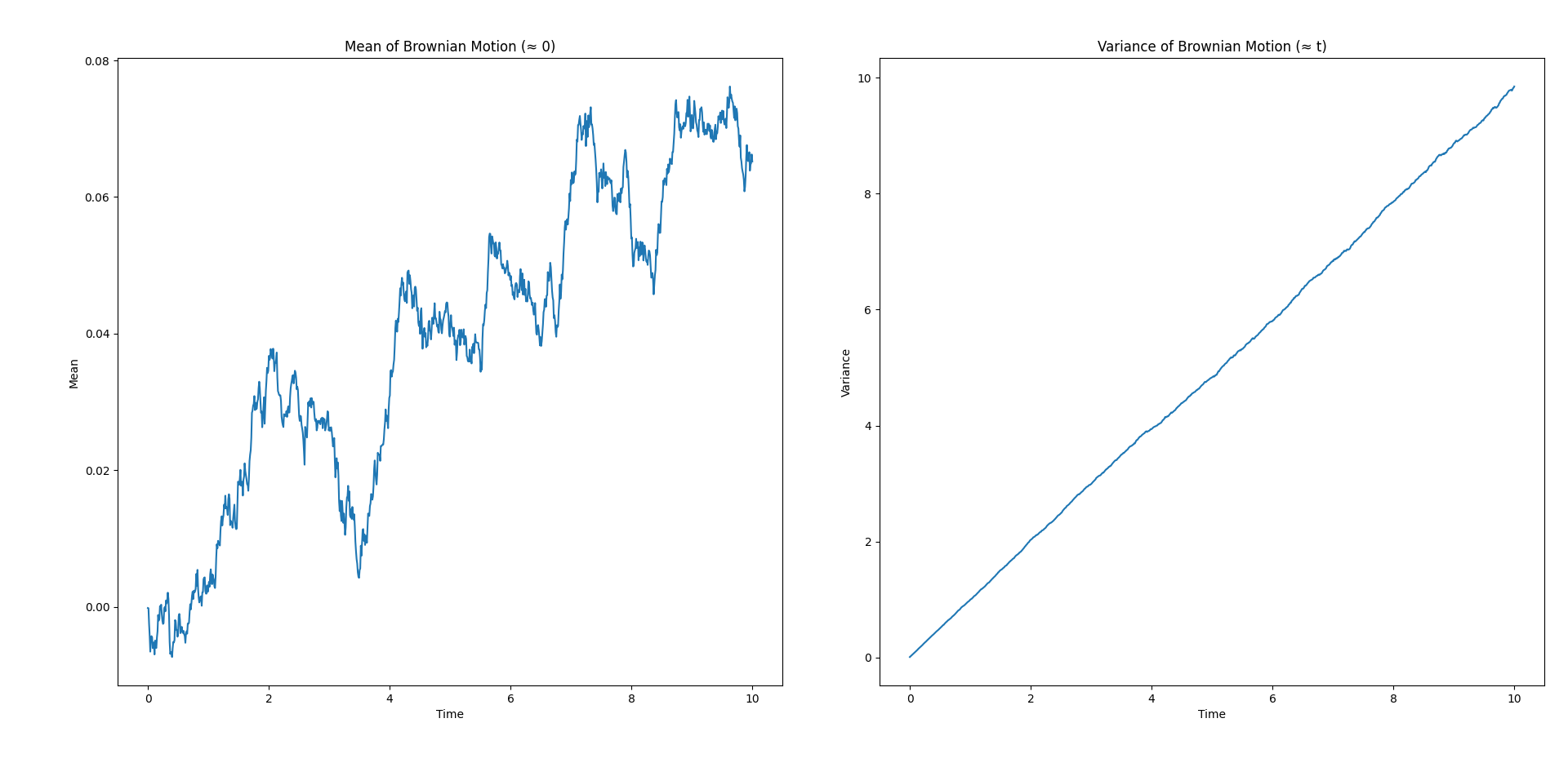
The left plot hovers around zero. The right one climbs in a nearly straight line — proof that randomness, averaged over time, behaves predictably.
Once you can model random change, the world opens up:
Stock prices fluctuate unpredictably; stochastic calculus powers the Black–Scholes model, which prices options based on this randomness.
The jiggling of pollen grains, the experiment that first revealed Brownian motion helped confirm the existence of atoms.
Anywhere uncertainty matters, stochastic calculus gives it structure.
At first glance, randomness looks like disorder — meaningless motion, unpredictable noise. But when you zoom out, patterns emerge. Averages stabilize. Variances follow laws. The drunkard’s walk becomes a mathematical universe:
A way to predict the unpredictable, measure the immeasurable, and understand the restless patterns that drive everything from markets to molecules.
That’s stochastic calculus — calculus for a world that never stops shaking.
✨ The Weekly Market Sentiment Report is evolving into The Signal Beyond 🚀.
This isn’t just a sentiment check anymore. It’s becoming a full market intelligence package with expanded technical scorecards, refined sentiment models, and machine learning forecasts. From classic tools that have stood the test of time to fresh innovations like multi-market RSI heatmaps, volatility regime dashboards, and pairs trading recommendation system, the new report is designed to give you a sharper edge in navigating the markets.
Free trial available.