Combinations of technical indicators may yield interesting results in market prediction methods. This article shows how to combine the adaptive moving average with the distance method in order to create an adaptive distance indicator.
Kauffman Adaptive Moving Average
The Kaufman adaptive moving average (KAMA) is a type of moving average used in technical analysis. It’s designed to adapt to changing market conditions, making it more responsive to recent price action. Unlike traditional moving averages that use fixed time periods, KAMA adjusts its sensitivity based on market volatility.
Here’s the basic idea: In volatile markets, KAMA reacts more quickly to price changes, helping you avoid false signals. In calmer markets, it becomes less sensitive to prevent unnecessary whipsaws. The adaptation is achieved by considering the efficiency ratio, which compares the price change to the overall price range. If the market is more volatile, the efficiency ratio increases, and KAMA becomes more responsive.
In simpler terms, KAMA is like a moving average that smartly adjusts itself according to how fast or slow prices are moving. This adaptability is meant to make it more effective in different market conditions, providing a smoother trend-following tool.
The following chart shows KAMA in action.
If you want to see more of my work, you can visit my website for the books catalogue by simply following this link:
Creating the Adaptive Distance Indicator
The distance method is when you calculate the difference between the close price and an overlay indicator (such as a moving average). This distance may show periods where the market is very far from normality and hence, a contrarian reaction may be imminent.
The adaptive distance indicator will follow this logic. It is constructed as follows:
Calculate an adaptive moving average.
Calculate the difference (distance) between the close price and the adaptive moving average.
Calculate a simple moving average on the difference from the previous step.
Calculate an upper and lower band on the previous step using the Bollinger bands principle.
Now, to generate signals you have to create basic rules. The following are the conditions for the signals:
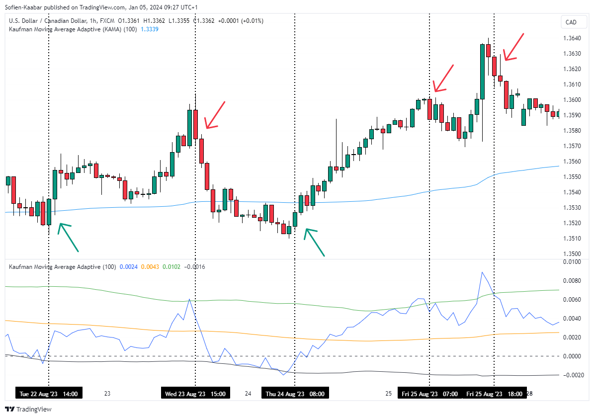
A bullish signal is generated whenever the indicator re-integrates the black line (the lower band).
A bearish signal is generated whenever the indicator re-integrates the green line (the upper band).
The following shows an example of the signals.
// This Pine Script™ code is subject to the terms of the Mozilla Public License 2.0 at https://mozilla.org/MPL/2.0/
// © Sofien-Kaabar

//@version=5
indicator("Kaufman Moving Average Adaptive", overlay = false)
Length = input(defval = 21, title = 'Lookback')
xPrice = close
xvnoise = math.abs(xPrice - xPrice[1])
nAMA = 0.0
nfastend = 0.666
nslowend = 0.0645
nsignal = math.abs(xPrice - xPrice[Length])
nnoise = math.sum(xvnoise, Length)
nefratio = nnoise != 0? nsignal / nnoise: 0
nsmooth = math.pow(nefratio * (nfastend - nslowend) + nslowend, 2)
nAMA := nz(nAMA[1]) + nsmooth * (xPrice - nz(nAMA[1]))

distance = close - nAMA
special_ma = ta.sma(distance, Length)
special_std = ta.stdev(distance, Length)

upper = special_ma + (2 * special_std)
lower = special_ma - (2 * special_std)

plot(distance)
plot(special_ma, color = color.orange)
plot(upper, color = color.green)
plot(lower, color = color.black)
hline(0, color = color.black)
The following shows more signals.
Another interesting method to use here is to wait for a pull-back before taking the position. For a bullish trade (shown below), the fact of re-integrating the orange line is not enough, the indicator must shape a pull-back to the black line to validate the signal.
The indicator looks stationary when zoomed out, as can be seen in the following chart.
We can create a simple signal algorithm that searches for successive pull-backs as follows:
// This Pine Script™ code is subject to the terms of the Mozilla Public License 2.0 at https://mozilla.org/MPL/2.0/
// © Sofien-Kaabar

//@version=5
indicator("Kaufman Moving Average Adaptive - Signals", overlay = true)

Length = input(defval = 21, title = 'Lookback')
xPrice = close

xvnoise = math.abs(xPrice - xPrice[1])
nAMA = 0.0
nfastend = 0.666
nslowend = 0.0645
nsignal = math.abs(xPrice - xPrice[Length])
nnoise = math.sum(xvnoise, Length)
nefratio = nnoise != 0? nsignal / nnoise: 0
nsmooth = math.pow(nefratio * (nfastend - nslowend) + nslowend, 2)
nAMA := nz(nAMA[1]) + nsmooth * (xPrice - nz(nAMA[1]))

distance = close - nAMA
special_ma = ta.sma(distance, Length)
special_std = ta.stdev(distance, Length)
upper = special_ma + (2 * special_std)
lower = special_ma - (2 * special_std)

bullish_signal = distance > lower and distance[1] > distance and distance[2] < lower[2]
bearish_signal = distance < upper and distance[1] < distance and distance[2] > upper[2]

plotshape(bullish_signal,  style = shape.triangleup, color = color.green, location =  location.belowbar, size = size.small)
plotshape(bearish_signal,  style = shape.triangledown, color = color.red, location =  location.abovebar, size = size.small)


