Simple Machine Learning Models for Time Series - The Tweedie Regression

Machine Learning Models for Time Series Analysis

This article will discuss a machine learning model referred to as Tweedie Regression. We will download a time series from an online source, transform it (i.e. make it stationary) and will simply apply the model’s tools to forecast t+1 values at each time step. We will just apply a simple performance evaluation tool, that is the accuracy (or hit ratio).

---

Intuition of the Model

The Tweedie Regressor is a type of regression model used when your target variable follows a Tweedie distribution—a flexible family of probability distributions that includes several well-known ones as special cases.

The Tweedie distribution is a compound Poisson-Gamma distribution, and it’s controlled by a parameter called the power parameter (p). Depending on the value of p, you get different distributions:

• p = 0 —> Normal

• p = 1 —> Poisson

• 1 < p < 2 —> Compound Poisson-Gamma

• p = 2 —> Gamma

• p = 3 —> Inverse Gaussian

The range 1 < p < 2 is the most commonly used in insurance and risk modeling, where the target is zero-inflated and positive-continuous (e.g., claim amounts: many zeros, and some large continuous values).

In machine learning (precisely, sklearn.linear_model.TweedieRegressor), the Tweedie Regressor fits a generalized linear model (GLM) assuming the target variable follows a Tweedie distribution.

It has three main inputs:

• power – the Tweedie power parameter described above.

• link – the link function, usually "log" for positive-valued data.

• alpha – regularization strength.

Do you want to master Deep Learning techniques tailored for time series, trading, and market analysis🔥? My book breaks it all down from basic machine learning to complex multi-period LSTM forecasting while going through concepts such as fractional differentiation and forecasting thresholds. Get your copy here 📖!

---

Using the Model to Forecast Time Series

Let’s use the model in Python to apply the returns of a time series. We’ll choose the returns of S&P 500 for this task, while knowing that it’s almost impossible to accurately predict such a chaotic dataset with simple models, but we will do it just to make the models work. The plan of attack is as follows:

• Download the time series.

• Take the returns of the prices to make it stationary (an important condition of machine learning forecasting).

• Split the data into training and test sets.

• Fit and predict.

• Evaluate and plot the predictions.

Use the following code to conduct the experiment.

from sklearn.linear_model import TweedieRegressor
import pandas_datareader as pdr
import numpy as np
import matplotlib.pyplot as plt

def data_preprocessing(data, num_lags, train_test_split):
    # Prepare the data for training
    x = []
    y = []
    for i in range(len(data) - num_lags):
        x.append(data[i:i + num_lags])
        y.append(data[i+ num_lags])
    # Convert the data to numpy arrays
    x = np.array(x)
    y = np.array(y)
    # Split the data into training and testing sets
    split_index = int(train_test_split * len(x))
    x_train = x[:split_index]
    y_train = y[:split_index]
    x_test = x[split_index:]
    y_test = y[split_index:]
    return x_train, y_train, x_test, y_test 

start_date = '1960-01-01'
end_date   = '2020-01-01'

# Import the data
data = (pdr.get_data_fred('SP500', start = start_date, end = end_date).dropna())
data = np.diff(data['SP500'])

# Train-test split
x_train, y_train, x_test, y_test = data_preprocessing(data, 100, 0.80)

# Create and train the model
model = TweedieRegressor()
model.fit(x_train, y_train)

# Make predictions on the test set
y_pred = model.predict(x_test)

# Evaluate the model
same_sign_count = np.sum(np.sign(y_pred) == np.sign(y_test)) / len(y_test) * 100
print('Hit Ratio = ', same_sign_count, '%')

# Plot the actual vs. predicted values
plt.figure(figsize=(12, 6))
plt.plot(y_test[-50:], label = 'Actual', color = 'blue')
plt.plot(y_pred[-50:], label = 'Predicted', color = 'red')
plt.legend()
plt.title('Actual vs. Predicted')
plt.ylabel('Value')
plt.show()
plt.grid()
plt.axhline(y = 0, color = 'black')

The following is the plot that compares the real data from the test set and the predicted data.

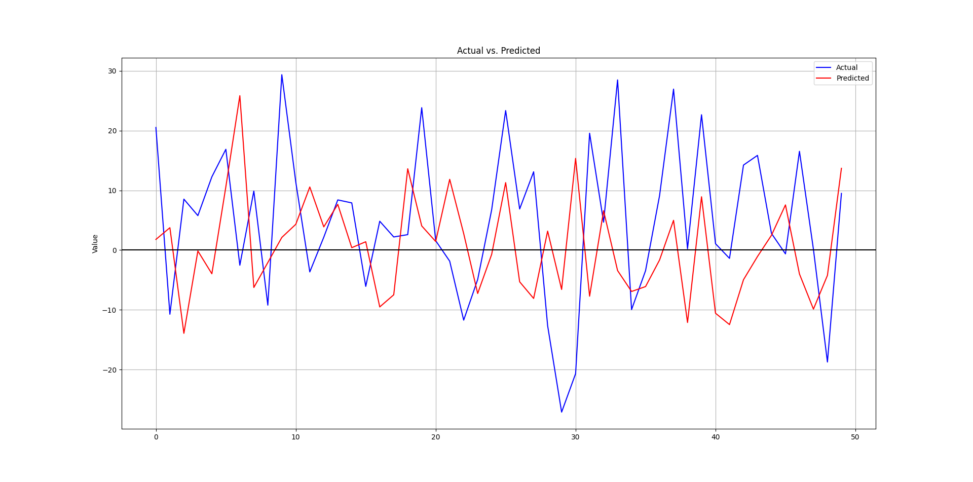
The following output shows the hit ratio.

44.60%

Every week, I analyze positioning, sentiment, and market structure. Curious what hedge funds, retail, and smart money are doing each week? Then join hundreds of readers here in the Weekly Market Sentiment Report 📜 and stay ahead of the game through chart forecasts, sentiment analysis, volatility diagnosis, and seasonality charts.

Free trial available🆓