


In this series, we will present Quantitative Research, a highly complex field where complex mathematical tools are used to deliver predictive value with regards to data (particularly, time series).
The aim of the series is to get you exposed to the key parts of quantitative research and its wide array of possibilities.
What Stationarity Actually Means
If probability distributions define what you assume about randomness, stationarity defines whether those assumptions survive time.
Most statistical models silently assume stationarity. Markets quietly violate it.
That mismatch is responsible for a massive share of model failure, false confidence, and blown strategies. This part is not optional. If you misunderstand stationarity, everything built on top of it is fragile.
A time series is stationary if its statistical properties do not change over time.
Formally, a process Xt is strictly stationary if the joint distribution satisfies:

That definition is elegant. It is also completely unrealistic for financial markets.
Weak (Second Order) Stationarity
In practice, quants work with weak stationarity. A process is weakly stationary if:
E[Xt] = μ is constant
Var(Xt) = σ2 is constant
Cov(Xt, Xt+k) depends only on k, not on t.
This is the version most models rely on. And even this weaker form is often violated.
Prices contain:
Trends
Inflation
Structural breaks
Growth components
Mathematically, prices often behave like:

This is a random walk, which is non stationary. Mean and variance explode over time. Let’s simulate a random walk in Python.
import numpy as np
import matplotlib.pyplot as plt

np.random.seed(0)

eps = np.random.normal(0, 1, 1000)
price = np.cumsum(eps)

plt.plot(price)
plt.title('Random Walk Price')
plt.show()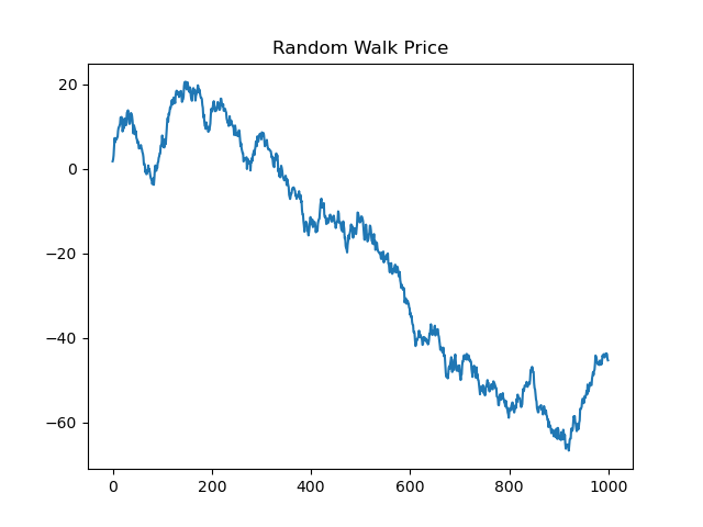
You cannot model this with stationary assumptions without transforming it.
The Signal Beyond 🚀
From classic tools that have stood the test of time to fresh innovations like multi-market RSI heatmaps, COT reports, seasonality, and pairs trading recommendation system, the new report is designed to give you a sharper edge in navigating the markets.
Free trial available.
Returns Are Closer to Stationary
Returns are typically defined as:

Returns remove the unit root in prices. They are closer to stationary, but still exhibit:
Volatility clustering
Changing higher moments
Regime dependence
This means:
Mean may be stable
Variance is not
Volatility is time varying by nature. This violates constant variance assumptions directly. This is why:
OLS breaks
Confidence intervals lie
Risk models understate drawdowns
returns = np.random.normal(0, 0.01, 1000)
returns[300:600] *= 4  # volatility regime

plt.plot(returns)
plt.title('Returns with Volatility Regime Shift')
plt.show()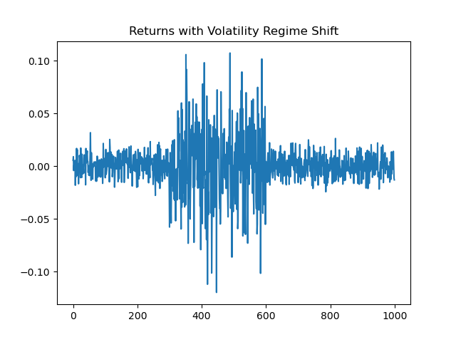
Same mean. Completely different risk.
Testing for Stationarity
Stationarity tests do not prove stationarity. They test for specific violations.
Augmented Dickey Fuller Test
Null hypothesis: unit root exists (non stationary).

from statsmodels.tsa.stattools import adfuller

result = adfuller(df['returns']) # you need a df
print('ADF Statistic:', result[0])
print('p-value:', result[1])
Low p-value does not mean safe forever.
KPSS Test
Null hypothesis: stationarity. Opposite of ADF.
from statsmodels.tsa.stattools import kpss

stat, p, _, _ = kpss(df['returns'])  # you need a df
print('KPSS Statistic:', stat)
print('p-value:', p)
Using both tests together is common.
Structural Breaks
Markets undergo structural changes:
Regulation
Technology
Liquidity
These breaks destroy stationarity instantly. Example:
Pre 2008 vs post 2008
Pre QE vs QE era
Low rate vs high rate regimes
A single model across both is conceptually invalid.
Regime Shifts
Markets operate in regimes with different statistical properties. Typical regimes:
Low volatility trend
High volatility trend
Mean reversion
Crisis
Each regime has its own:
Mean
Variance
Correlation structure
Tail behavior
Mixture Interpretation

Where st is a hidden regime state. This immediately invalidates single distribution assumptions.
Rolling Statistics as Reality Check
If statistics drift over time, stationarity is violated.
window = 100

rolling_mean = df['returns'].rolling(window).mean()
rolling_std = df['returns'].rolling(window).std()

plt.plot(rolling_mean, label='Rolling Mean')
plt.plot(rolling_std, label='Rolling Std')
plt.legend()
plt.show()
If these move materially, your model assumptions are outdated.
Differencing and Detrending
One common approach to enforce stationarity.
Differencing
Removes trends but:
Amplifies noise
Destroys long-term structure

Detrending
Remove deterministic trend components.
from scipy.signal import detrend

detrended = detrend(df['price'])
Be careful: you are injecting assumptions.
Do you want to master Deep Learning techniques tailored for time series, trading, and market analysis🔥?
My book breaks it all down from basic machine learning to complex multi-period LSTM forecasting while going through concepts such as fractional differentiation and forecasting thresholds.
Get your copy here 📖!