
Quantitative Research Part II - Probability Distributions in Finance
Introduction to Quantitative Research in a Simplified Way


In this series, we will present Quantitative Research, a highly complex field where complex mathematical tools are used to deliver predictive value with regards to data (particularly, time series).
The aim of the series is to get you exposed to the key parts of quantitative research and its wide array of possibilities.
Probability Distributions in Finance
If descriptive statistics tell you what the data looks like, probability distributions tell you what you assume about reality.
Every quantitative model makes distributional assumptions. Most of them are wrong. Many of them are dangerous.
This article explains probability distributions from a market reality perspective, not an academic one. You will learn what distributions are used, why they are used, where they fail, and how to work with them responsibly in Python.
Why Distributions Matter More Than Models
A model is just a transformation of assumptions. If your assumed distribution is wrong:
Risk is mispriced
Tail events are ignored
Signals look better than they are
Capital is destroyed quietly
Before regression, ML, or optimization, you must answer:
What is the probabilistic structure of my data?
Random Variables in Finance
A random variable maps outcomes to numbers. In finance:
Returns are random variables
Drawdowns are random variables
Volatility is a random variable
Time between crashes is a random variable
Discrete vs Continuous
Discrete: trade counts, tick moves, number of limit hits
Continuous: returns, prices, log prices, spreads
Most financial modeling uses continuous random variables, even when reality is discrete. This approximation already introduces error.
The Normal Distribution
A random variable X is normally distributed if:
Defined entirely by:
Mean μ
Standard deviation σ
The Signal Beyond 🚀
From classic tools that have stood the test of time to fresh innovations like multi-market RSI heatmaps, COT reports, seasonality, and pairs trading recommendation system, the new report is designed to give you a sharper edge in navigating the markets.
Free trial available.
Why the Normal Distribution Fails
Empirical returns exhibit:
Fat tails
Skewness
Volatility clustering
Extreme events far beyond Gaussian probability
A 5-sigma event should happen once in millions of years. Markets produce them every decade.
import numpy as np
np.random.seed(42)
n_days = 1000 # length of time series
mu = 0.0004 # daily drift (~10% annualized)
sigma = 0.01 # daily volatility (~16% annualized)
returns = np.random.normal(loc=mu, scale=sigma, size=n_days)
from scipy.stats import norm
import numpy as np
import matplotlib.pyplot as plt
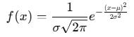
mu, sigma = np.mean(returns), np.std(returns)
x = np.linspace(returns.min(), returns.max(), 500)
plt.hist(returns, bins=50, density=True, alpha=0.6)
plt.plot(x, norm.pdf(x, mu, sigma))
plt.title('Gaussian Fit vs Empirical Returns')
plt.show()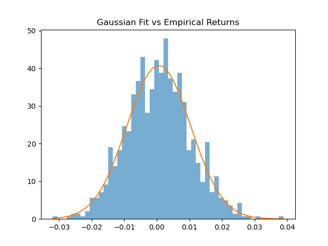
If this fit looks acceptable to you, you are not looking at the tails.
Fat-Tailed Distributions
Markets are leptokurtic. Tail behavior matters more than center behavior.
Student’s t Distribution
The Student’s t distribution is what you use when Gaussian assumptions break.
It looks like a normal distribution in the center and behaves very differently in the tails.
Where ν controls tail thickness.
Low ν → fat tails
High ν → Gaussian-like
from scipy.stats import t

df_hat, loc_hat, scale_hat = t.fit(returns)

plt.hist(returns, bins=50, density=True, alpha=0.6)
plt.plot(x, t.pdf(x, df_hat, loc_hat, scale_hat))
plt.title(”Student-t Fit to Returns”)
plt.show()
This already outperforms Gaussian assumptions in most markets.
Why t-Distributions Still Fall Short
Symmetric by default
Static tail thickness
No volatility clustering
No regime shifts
They are better. Not sufficient.
Skewed Distributions
Returns are rarely symmetric.
Skew-Normal Distribution
Adds a skewness parameter α. Useful for:
Option PnL
Carry trades
Trend-following returns
from scipy.stats import skewnorm

a, loc, scale = skewnorm.fit(returns)

plt.hist(returns, bins=50, density=True, alpha=0.6)
plt.plot(x, skewnorm.pdf(x, a, loc, scale))
plt.title(”Skew-Normal Fit”)
plt.show()
Still parametric. Still limited.
Empirical Distributions
The most honest distribution is the one you observe.
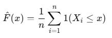
Empirical CDF
Empirical CDF (ECDF) is the data-driven version of a cumulative distribution function. No assumptions. No parametric model. Just the data.
sorted_r = np.sort(returns)
cdf = np.arange(1, len(sorted_r)+1) / len(sorted_r)

plt.plot(sorted_r, cdf)
plt.title(”Empirical CDF”)
plt.show()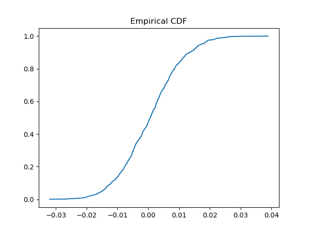
Empirical distributions are:
Noisy
Sample dependent
Honest about tails
Mixture Distributions and Regimes
Markets are not one distribution. They are multiple distributions switching over time.
Regime Mixtures
Examples:
Calm regime
Volatile regime
Crisis regime
regime1 = np.random.normal(0, 0.005, 700)
regime2 = np.random.normal(0, 0.03, 300)

mixed_returns = np.concatenate([regime1, regime2])
Single-distribution fitting hides this structure completely.
Conditional vs Unconditional Distributions
This distinction is critical.
Unconditional: full-sample distribution
Conditional: distribution given information
Examples:
Returns given high volatility
Returns given trend
Returns after drawdowns
Most alpha exists conditionally, not unconditionally.
Always ask: conditional on what?
Why Probability Assumptions Break Models
Let us be explicit.
Value-at-Risk fails due to tail assumptions
Sharpe ratios fail under skewness
Mean-variance optimization collapses under fat tails
Backtests lie when distributions shift
Distributional ignorance is the root cause.
Do you want to master Deep Learning techniques tailored for time series, trading, and market analysis🔥?
My book breaks it all down from basic machine learning to complex multi-period LSTM forecasting while going through concepts such as fractional differentiation and forecasting thresholds.
Get your copy here 📖!