
Quantitative Research Part I - Introduction to Descriptive Statistics
Introduction to Quantitative Research in a Simplified Way


In this series, we will present Quantitative Research, a highly complex field where complex mathematical tools are used to deliver predictive value with regards to data (particularly, time series).
The aim of the series is to get you exposed to the key parts of quantitative research and its wide array of possibilities.
A Primer on Descriptive Statistics
Quantitative research does not start with machine learning, neural networks, or fancy predictive models. It starts with describing reality correctly.
Before you forecast, optimize, or trade anything, you must understand what the data is, how it behaves, and what it hides. Descriptive statistics are not a beginner topic. They are the foundation that silently determines whether every downstream model succeeds or fails.
Most failed quant models fail here, not later.
What Descriptive Statistics Actually Do
Descriptive statistics answer a simple but brutal question:
What is the data doing, without pretending it is smarter than it is?
They summarize, compress, and structure information without inference.
No prediction. No causality. No hypothesis testing.
In quant research, descriptive statistics serve four roles:
Data sanity checking
Regime identification
Feature understanding
Model failure diagnosis
If you skip them, you are blind.
Types of Data You Will Encounter
Before computing anything, you must know what kind of data you are handling.
Cross-Sectional Data
Multiple assets at a single point in time.
Examples:
Stock returns today
Volatility across assets
Factor exposures
Time Series Data
One variable observed through time.
Examples:
Price
Returns
Volume
Indicators
This is where most quant work lives.
Panel Data
Multiple assets observed through time.
Examples:
Equity universes
FX baskets
Macro datasets
Almost all institutional research uses panel data.
Measures of Central Tendency
Central tendency answers the question:
Where does the data live?
Arithmetic Mean | The most abused statistic in finance
For a dataset x1, x2,..., xn:
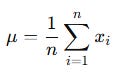
The mean assumes:
Symmetry
No extreme outliers
Finite variance
Markets violate all three.
import numpy as np

mean = np.mean(returns)
The mean of returns is often meaningless in fat-tailed distributions.
The Signal Beyond 🚀
From classic tools that have stood the test of time to fresh innovations like multi-market RSI heatmaps, COT reports, seasonality, and pairs trading recommendation system, the new report is designed to give you a sharper edge in navigating the markets.
Free trial available.
Median | The most underrated statistic
The median is the middle value after sorting. It’s important because it is
Robust to outliers
More stable across regimes
Better representative of typical behavior
median = np.median(returns)If mean and median diverge significantly, your distribution is skewed or polluted.
Mode | The most frequent value
Rarely useful for continuous financial data. Sometimes useful for discrete variables like trade sizes or tick data.
Measures of Dispersion
Central tendency without dispersion is useless. Dispersion answers:
How violent is the data?
Variance
The mathematical representation of variance is as follows:
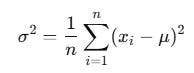
Variance penalizes large deviations heavily.
Python
variance = np.var(returns, ddof=1)Use ddof=1 for sample variance.
Standard Deviation | The square root of variance
This is what traders mistakenly call risk.
std = np.std(returns, ddof=1)Standard deviation assumes:
Normality
Linear risk
Symmetry
Markets do not care.
Range and Interquartile Range
The mathematical representation of the range is as follows:
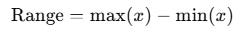
Useless alone. Dominated by outliers. The interquartile range (IQR) is as follows:
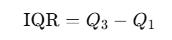
q1 = np.percentile(returns, 25)
q3 = np.percentile(returns, 75)
iqr = q3 - q1
IQR is your friend in noisy markets.
Shape of Distributions
This is where most quant intuition is born.
Skewness
Skewness measures asymmetry.
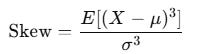
Positive skew: rare large gains
Negative skew: rare large losses
from scipy.stats import skew

sk = skew(returns)
Most strategies die from negative skew, not low Sharpe.
Kurtosis
Kurtosis measures tail heaviness.
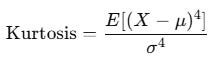
Normal distribution has kurtosis of 3. Finance usually has excess kurtosis.
from scipy.stats import kurtosis

kt = kurtosis(returns, fisher=False)
High kurtosis means tail risk is real, not theoretical.
Moments of a Distribution
Descriptive statistics are structured as moments:
First → Mean
Second → Variance
Third → Skewness
Fourth → Kurtosis
Most models implicitly assume only the first two matter. That assumption is usually wrong.
Robust Statistics
Markets are adversarial environments. Your statistics must survive abuse.
Trimmed Mean
Ignore extreme values.
from scipy.stats import trim_mean

trimmed = trim_mean(returns, 0.05)
Median Absolute Deviation
The formula for this is as follows:

mad = np.median(np.abs(returns - np.median(returns)))MAD beats standard deviation during crises.
Rolling Descriptive Statistics
Static statistics lie in non-stationary markets. Rolling statistics reveal regime changes.
window = 50

rolling_mean = returns.rolling(window).mean()
rolling_std = returns.rolling(window).std()
Let’s see all of this with an example:
import numpy as np
import pandas as pd
import matplotlib.pyplot as plt
from scipy.stats import skew, kurtosis

np.random.seed(42)

n_obs = 1000
dates = pd.date_range(start=”2020-01-01”, periods=n_obs, freq=”D”)

# Simulate returns with fat tails (Student-t)
df_t = 4
returns = 0.0005 + 0.01 * np.random.standard_t(df=df_t, size=n_obs)

# Convert returns to price series
price = 100 * np.exp(np.cumsum(returns))

df = pd.DataFrame(
    {
        “price”: price,
        “returns”: returns
    },
    index=dates
)

# Basic descriptive statistics
stats = {}

stats[”mean_return”] = df[”returns”].mean()
stats[”median_return”] = df[”returns”].median()
stats[”std_return”] = df[”returns”].std()
stats[”variance_return”] = df[”returns”].var()

stats[”min_return”] = df[”returns”].min()
stats[”max_return”] = df[”returns”].max()

stats[”skewness”] = skew(df[”returns”])
stats[”kurtosis”] = kurtosis(df[”returns”], fisher=False)

# Quantiles
stats[”q01”] = df[”returns”].quantile(0.01)
stats[”q05”] = df[”returns”].quantile(0.05)
stats[”q95”] = df[”returns”].quantile(0.95)
stats[”q99”] = df[”returns”].quantile(0.99)

# Robust statistics
median = df[”returns”].median()
mad = np.median(np.abs(df[”returns”] - median))
iqr = df[”returns”].quantile(0.75) - df[”returns”].quantile(0.25)

stats[”MAD”] = mad
stats[”IQR”] = iqr


# Rolling statistics (regime awareness)
window = 50

df[”rolling_mean”] = df[”returns”].rolling(window).mean()
df[”rolling_std”] = df[”returns”].rolling(window).std()

print(”\nDESCRIPTIVE STATISTICS (RETURNS)\n”)

for k, v in stats.items():
    print(f”{k:20s}: {v: .6f}”)

# Visualization
plt.figure(figsize=(12, 5))
plt.plot(df.index, df[”price”])
plt.title(”Hypothetical Price Time Series”)
plt.xlabel(”Date”)
plt.ylabel(”Price”)
plt.show()

plt.figure(figsize=(12, 5))
plt.hist(df[”returns”], bins=50)
plt.title(”Return Distribution (Fat Tails)”)
plt.xlabel(”Returns”)
plt.ylabel(”Frequency”)
plt.show()

plt.figure(figsize=(12, 5))
plt.plot(df.index, df[”rolling_std”])
plt.title(”Rolling Volatility (50-day)”)
plt.xlabel(”Date”)
plt.ylabel(”Rolling Std”)
plt.show()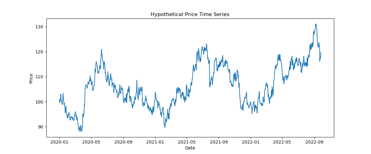
mean_return         :  0.000180
median_return       :  0.000315
std_return          :  0.013085
variance_return     :  0.000171
min_return          : -0.095929
max_return          :  0.061775
skewness            : -0.335217
kurtosis            :  7.439154
q01                 : -0.034367
q05                 : -0.020559
q95                 :  0.020284
q99                 :  0.036200
MAD                 :  0.007211
IQR                 :  0.014354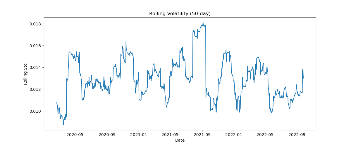
Do you want to master Deep Learning techniques tailored for time series, trading, and market analysis🔥?
My book breaks it all down from basic machine learning to complex multi-period LSTM forecasting while going through concepts such as fractional differentiation and forecasting thresholds.
Get your copy here 📖!