Quantifying Market Psychology -Part III
A Systematic Research on Psychological Levels in the FX Market
This article expands on the concets seen in part two of the series: Quantifying Market Psychology. Please refer to the second part before reading this article.
The RSI
Created by J. Welles Wilder Jr., The Relative Strength Index (RSI) is one of the pillars of technical indicators. It is mainly used for contrarian signals, where extreme values hint at a possible market reaction. Typically, we use the following steps to calculate the RSI:
· Calculate the change in the close prices from the previous ones.
· Separate the positive net changes from the negative net changes.
· Calculate a smoothed moving average[2] on the positive net changes and on the absolute values of the negative net changes.
· Divide the smoothed positive changes by the smoothed negative changes. We will refer to this calculation as the Relative Strength (RS).
Apply the normalization formula shown below for every time step to get the RSI.
Although 14 is the default lookback period on the RSI, we will be back-testing 5 as a lookback period as it provides more statistically significant results.
Figure 11: EURAUD hourly data with a 5-period RSI
Combining the PLS With the RSI
Typically, we use 30 as an oversold level and 70 as an overbought level when looking at the RSI.
This means that whenever the RSI reaches 30, the expectation is that there should soon be a market bounce as the momentum is considered to be too negative and ready for a change.
In parallel, whenever the RSI reaches 70, the expectation is that there should soon be a market pause soon as the momentum is considered to be too positive.
The trading conditions of the strategy are as follows:
Bullish Signal
The bullish PLS signal requires the 5-period RSI to be at or below 30.
Bearish Signal
The bearish PLS signal requires the 5-period RSI to be at or above 70.
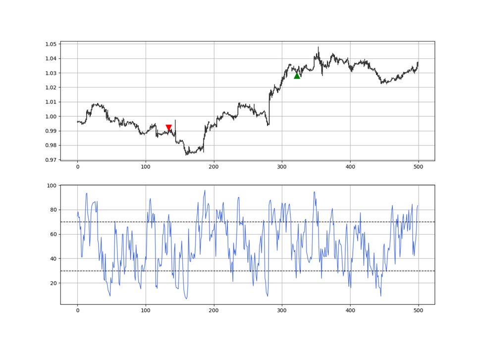
Figure 12: A signal chart illustrating the RSI-filtered PLS applied on EURUSD
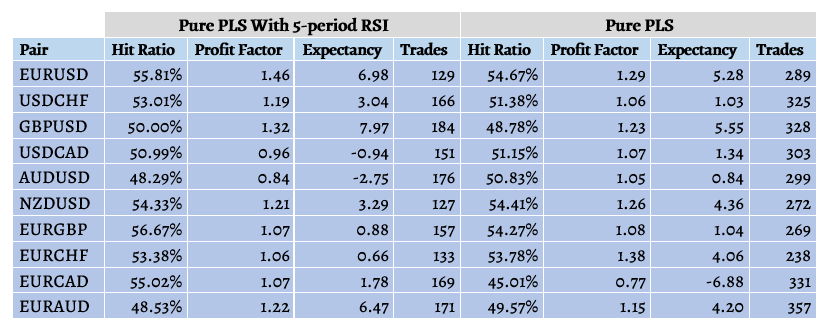
The simplest way to detect the added value of the RSI is to compare the evolution of the results between the pure PLS and the RSI-filtered PLS.
Table 10: Performance summary table of the RSI-filtered PLS and the pure PLS
The RSI strategy outperforms on five currency pairs and underperforms on the remaining five. This is seen across the performance metrics. However, the number of trades is halved when taking into account the RSI filter which shows a clear added value with regards to transaction costs.
In conclusion, it seems that the RSI’s filter does not impact much the profitability but does seem to remove around 50% of the trades which could significantly reduce the transaction costs incurred with each trade.
Bollinger Bands
Volatility plays an important role in financial markets. It represents risk when seen from a portfolio management perspective but can also represent opportunity from a trading perspective. John Bollinger created his famous Bollinger Bands using the mean and the standard deviation of the market price to create a moving envelope that contains most market variations.
In other words, Bollinger bands are a set of dynamic (moving) support and resistance levels that are said to add tremendous value during ranging markets. The steps needed to create the bands are as follows:
· Calculate a 20-period moving average on the close prices.
· Calculate a 20-period moving standard deviation on the close prices and multiply each result by 2.
· To find the upper Bollinger band which represents resistance, we add the current value of the moving average to the current value of the moving standard deviation.
· To find the lower Bollinger band which represents support, we subtract the current value of the moving average from the current value of the moving standard deviation.
According to the normal distribution, 95% of data lie within two standard deviations of their mean. It is a known fact that financial returns (and even more prices) do not follow a normal distribution, but we tend to compare them to the normal distribution as an approximation.
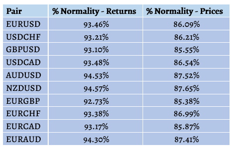
If we consider taking the percentage of times where the market was higher than its lower Bollinger band and lower than its upper Bollinger band, we will found that it hovers around 86% for hourly data of the observed currency pairs. Bollinger bands are based on prices and the normality condition implies that around 86% of the market price of the followed currency pairs should lie within this implied statistical normality.
Table 11: Percentage of times where returns and prices fall above their lower Bollinger band and below their upper Bollinger band.
Naturally, the previous table only takes into account the last 20 periods for each calculation as it tries to understand the efficacy of the Bollinger bands.
In comparison, if we do the same calculation for the returns instead of prices, we find that it is closer to normality which is in tandem with the theoretical results which state that financial returns may be stationary (stable mean and variance across time) but financial prices are certainly non-stationary.
The implication of this is that 14% of the time, we will have a chance of finding a psychological level and applying the strategy on it. This already gives a clue as to severe filtering effect we will have since the signals will be given when the market is outside the bands (i.e. lower than the lower band or higher than the upper band).
Figure 13: EURUSD hourly data with the Bollinger bands
Combining the PLS With Bollinger Bands
The trading conditions of the Bollinger-filtered PLS are as follows:
Bullish Signal
The bullish PLS signal requires the market price at entry to be below the lower Bollinger band.
Bearish Signal
The bullish PLS signal requires the market price at entry to be above the upper Bollinger band.
Figure 14: A signal chart illustrating the Bollinger-filtered PLS applied on GBPUSD
Table 12: Performance summary table of the Bollinger-filtered PLS and the pure PLS
Similar to the RSI, it looks like the Bollinger bands are doing a better job filtering the trades while sacrificing some but not all returns. This can be seen as a cost optimization technique but undoubtedly not a performance enhancer.
The trades from the Bollinger filter represent around 24% of the trades from the pure PLS which is a tremendous decline in frequency and therefore in transaction costs.
If we take the example of the EURUSD’s back-test, we notice that the expectancy metric is cut in half while the number of trades are cut in five and represent 20% of the pure PLS trades which can present an opportunity of lowering the risk and the transaction costs while sacrificing less return.


