Passive Aggressive Regression Model for Time Series

Step-by-Step Guide to Create a Passive Aggressive Machine Learning Model

Passive aggressive regression (PAR) is a type of online learning algorithm used for regression tasks. It is part of the passive-aggressive (PA) algorithms, which are a family of machine learning methods designed for online learning—where data comes in sequentially rather than all at once.

This article presents this model and creates a time series forecasting algorithm in Python.

Passive Aggressive Algorithm

Passive means if the prediction is correct or the error is small, the model does not change much. Aggressive means if the prediction is incorrect, the model updates itself aggressively to correct the error.

This makes PAR ideal for real-time, continuously updated datasets, such as financial markets, stock price predictions, or streaming data. It has many characteristics:

• It updates the model incrementally as new data arrives.

• Unlike traditional regression (like linear regression), it does not need all data at once.

• Suitable for large datasets or real-time applications.

• The model updates itself only when the error exceeds a certain threshold.

PAR is similar to support vector regression but works in an online learning setting.

Given a dataset with input X and target Y, the objective function for PAR is:

subject to the constraint:

If the absolute error exceeds the margin of tolerance, the weight vector is updated as:

It’s important to know when to use this model:

✅ When data arrives in a stream (real-time updates needed).
✅ When handling large datasets that do not fit in memory.
✅ When model updates should be efficient and incremental.
✅ When working with non-stationary data, e.g., financial markets, demand forecasting.

Creating the Model

Let’s create the model in Python by importing data and the required libraries. We will use as data the US core consumer price index (CPI).

✨ Important note

Why make the data stationary? Making the data stationary before forecasting is important because many time series forecasting techniques assume that the underlying data generating process is stationary. Stationarity refers to the statistical properties of a time series remaining constant over time.

Use the following code to implement the task:

# Importing libraries
from sklearn import linear_model
import numpy as np
import matplotlib.pyplot as plt
import pandas_datareader as pdr

# Set the start and end dates for the data
start_date = '1980-01-01'
end_date   = '2024-02-01'
# Fetch the CPI data
data = np.array((pdr.get_data_fred('CPILFESL', start = start_date, end = end_date)).dropna())
# Difference the data and make it stationary
data = np.diff(data[:, 0])
data = np.diff(data[:])
# Setting the hyperparameters
num_lags = 100
train_test_split = 0.80
def data_preprocessing(data, num_lags, train_test_split):
    # Prepare the data for training
    x = []
    y = []
    for i in range(len(data) - num_lags):
        x.append(data[i:i + num_lags])
        y.append(data[i+ num_lags])
    # Convert the data to numpy arrays
    x = np.array(x)
    y = np.array(y)
    # Split the data into training and testing sets
    split_index = int(train_test_split * len(x))
    x_train = x[:split_index]
    y_train = y[:split_index]
    x_test = x[split_index:]
    y_test = y[split_index:]
    
    return x_train, y_train, x_test, y_test 
# Creating the training and test sets
x_train, y_train, x_test, y_test = data_preprocessing(data, num_lags, train_test_split)
model = linear_model.PassiveAggressiveRegressor()
# Train the model
model.fit(x_train, y_train)
# Predicting out-of-sample
y_pred = np.reshape(model.predict(x_test), (-1))
# Plotting
plt.plot(y_pred[-100:], label='Predicted Data', linestyle='--', marker = '.', color = 'red')
plt.plot(y_test[-100:], label='True Data', marker = '.', alpha = 0.7, color = 'blue')
plt.legend()
plt.grid()
plt.axhline(y = 0, color = 'black', linestyle = '--')
same_sign_count = np.sum(np.sign(y_pred) == np.sign(y_test)) / len(y_test) * 100
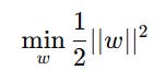
print('Hit Ratio = ', same_sign_count, '%')

The following chart shows the predicted data (red) compared to real data. The hit ratio was about 68%.

Check out my newsletter that sends weekly directional views every weekend to highlight the important trading opportunities using a mix between sentiment analysis (COT report, put-call ratio, etc.) and rules-based technical analysis.

With that being said, PAR algorithms have the following characteristics:

✔ Works well with large-scale, high-dimensional data
✔ Does not require batch training (online learning approach)
✔ Efficient updates for real-time learning
✔ Automatically adapts to new patterns in the data

In the meantime, they have the following cons:

❌ Not ideal for static datasets.
❌ Sensitive to hyperparameter.
❌ Assumes a linear relationship, which may not work well for complex, non-linear problems

PAR is an excellent choice when dealing with streaming, non-stationary data that requires real-time updates. It is fast, scalable, and effective, but requires careful tuning of hyperparameters to achieve optimal performance. If your dataset is static or requires a complex, non-linear relationship, then alternatives like random forests or neural networks might be better.