


Modern Contrarian Trading Strategies in Python — Part I.
Creating a Strategy Based on the RSI² Indicator.


The quest for the ultimate trading strategies is filled with unlimited opportunities and combinations. We always have to dig deeper to find opportunities that have not been exploited yet. Consider a goldmine with many miners, soon it will have no nuggets left. This can be compared to trading strategies where crowded ones have stopped working. This article discusses one exotic strategy that is not very known.
I have just published a new book after the success of my previous one “New Technical Indicators in Python”. It features a more complete description and addition of structured trading strategies with a Github page dedicated to the continuously updated code. If you feel that this interests you, feel free to visit the below link, or if you prefer to buy the PDF version, you could contact me on LinkedIn.
The Book of Trading Strategies
Amazon.com: The Book of Trading Strategies: 9798532885707: Kaabar, Sofien: Bookswww.amazon.com
The Relative Strength Index
The RSI is without a doubt the most famous momentum indicator out there, and this is to be expected as it has many strengths especially in ranging markets. It is also bounded between 0 and 100 which makes it easier to interpret. Also, the fact that it is famous, contributes to its potential.
This is because the more traders and portfolio managers look at the RSI, the more people will react based on its signals and this in turn can push market prices. Of course, we cannot prove this idea, but it is intuitive as one of the basis of Technical Analysis is that it is self-fulfilling.
The RSI is calculated using a rather simple way. We first start by taking price differences of one period. This means that we have to subtract every closing price from the one before it. Then, we will calculate the smoothed average of the positive differences and divide it by the smoothed average of the negative differences. The last calculation gives us the Relative Strength which is then used in the RSI formula to be transformed into a measure between 0 and 100.
To calculate the Relative Strength Index, we need an OHLC array (not a data frame). This means that we will be looking at an array of 4 columns. The function for the Relative Strength Index is therefore:
def adder(Data, times):

    for i in range(1, times + 1):

        new = np.zeros((len(Data), 1), dtype = float)
        Data = np.append(Data, new, axis = 1)
    return Data
def deleter(Data, index, times):

    for i in range(1, times + 1):

        Data = np.delete(Data, index, axis = 1)
    return Data

def jump(Data, jump):

    Data = Data[jump:, ]

    return Datadef ma(Data, lookback, close, where):

    Data = adder(Data, 1)

    for i in range(len(Data)):

            try:
                Data[i, where] = (Data[i - lookback + 1:i + 1, close].mean())

            except IndexError:
                pass

    # Cleaning
    Data = jump(Data, lookback)

    return Datadef ema(Data, alpha, lookback, what, where):

    alpha = alpha / (lookback + 1.0)
    beta  = 1 - alpha

    # First value is a simple SMA
    Data = ma(Data, lookback, what, where)

    # Calculating first EMA
    Data[lookback + 1, where] = (Data[lookback + 1, what] * alpha) + (Data[lookback, where] * beta)

    # Calculating the rest of EMA
    for i in range(lookback + 2, len(Data)):
            try:
                Data[i, where] = (Data[i, what] * alpha) + (Data[i - 1, where] * beta)

            except IndexError:
                pass

    return Data
def rsi(Data, lookback, close, where, width = 1, genre = 'Smoothed'):

    # Adding a few columns
    Data = adder(Data, 7)

    # Calculating Differences
    for i in range(len(Data)):

        Data[i, where] = Data[i, close] - Data[i - width, close]

    # Calculating the Up and Down absolute values
    for i in range(len(Data)):

        if Data[i, where] > 0:

            Data[i, where + 1] = Data[i, where]

        elif Data[i, where] < 0:

            Data[i, where + 2] = abs(Data[i, where])

    # Calculating the Smoothed Moving Average on Up and Down
    absolute values
    if genre == 'Smoothed':
      lookback = (lookback * 2) - 1 # From exponential to smoothed
      Data = ema(Data, 2, lookback, where + 1, where + 3)
      Data = ema(Data, 2, lookback, where + 2, where + 4)

    if genre == 'Simple':
      Data = ma(Data, lookback, where + 1, where + 3)
      Data = ma(Data, lookback, where + 2, where + 4)

    # Calculating the Relative Strength
    Data[:, where + 5] = Data[:, where + 3] / Data[:, where + 4]

    # Calculate the Relative Strength Index
    Data[:, where + 6] = (100 - (100 / (1 + Data[:, where + 5])))

    # Cleaning
    Data = deleter(Data, where, 6)
    Data = jump(Data, lookback)
    return Data
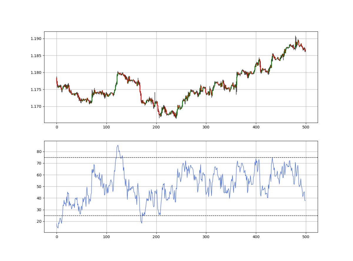
The Relative Strength Index is known for the extremes strategy (Oversold and Overbought levels) where we initiate contrarian positions when the RSI is close to the extremes in an attempt to fade the current trend.
The RSI²
The RSI² is a very simple idea. The hypothesis is that the RSI is a stationary indicator and is more easily forecasted than the actual price chart. Hence, we apply an RSI to the RSI so that we use the second RSI (Which we call RSI²) to forecast the direction of the original RSI. Why do we do this? Because historically, the correlation between the market return and its own RSI (Change in value) is very high.

The limitations of this strategy is that we are using a transformation of a price-transformation indicator to predict semi-random data. This gives a huge weight to lift. Therefore, we will be running our strategy based on the intuition above with certain conditions that make it less prone to lag.
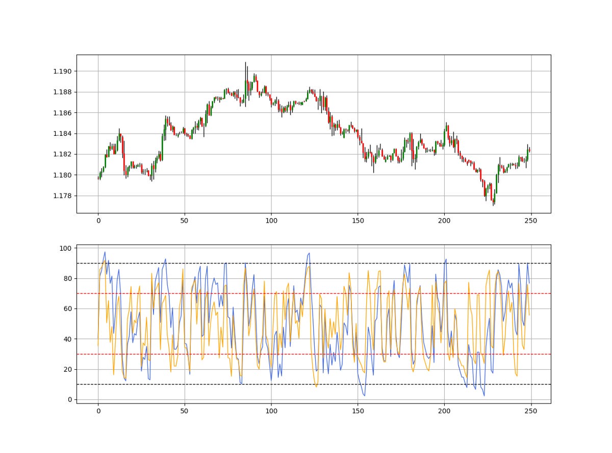
The Relative Strength Index is known for the extremes strategy (Oversold and Overbought levels) where we initiate contrarian positions when the RSI is close to the extremes in an attempt to fade the current trend. We will be using this technique applied on both RSI’s with unconventional lookback periods.
Whenever the 3-period RSI is at or below 10 while simultaneously, the 3-period RSI² is also at or below 30, we can expect a limited bullish reaction.
Whenever the 3-period RSI is at or above 90 while simultaneously, the 3-period RSI² is also at or above 70, we can expect a limited bearish reaction.
If you are also interested by more technical indicators and using Python to create strategies, then my best-selling book on Technical Indicators may interest you:
New Technical Indicators in Python
Amazon.com: New Technical Indicators in Python: 9798711128861: Kaabar, Mr Sofien: Bookswww.amazon.com
Creating the Strategy
Our aim is clear. We have to find double oversold/overbought events where we reinforce the conviction by saying that even the RSI on RSI is on the extreme which can argue that the RSI is truly on the extremes.
# Indicator Parameters
lookback = 3
lower_barrier = 10
upper_barrier = 90 lower_barrier_square = 30
upper_barrier_square = 70 my_data = adder(my_data, 10)
my_data = rsi(my_data, lookback, 3, 4)
my_data = rsi(my_data, lookback, 4, 5)
The signal function that we need can be as follows.
def signal(Data, indicator_column_one, indicator_column_two, buy, sell):

    Data = adder(Data, 10)

    for i in range(len(Data)):

        if Data[i, indicator_column_one] <= lower_barrier and Data[i, indicator_column_two] <= lower_barrier_square and \
            Data[i - 1, indicator_column_one] > lower_barrier:
            Data[i, buy] = 1

        elif Data[i, indicator_column_one] >= upper_barrier and Data[i, indicator_column_two] >= upper_barrier_square and \
            Data[i - 1, indicator_column_one] < upper_barrier:
            Data[i, sell] = -1

    return Data
Evaluating the Strategy
Having had the signals, we now know when the algorithm would have placed its buy and sell orders, meaning, that we have an approximate replica of the past where can can control our decisions with no hindsight bias. We have to simulate how the strategy would have done given our conditions. This means that we need to calculate the returns and analyze the performance metrics. Let us see a neutral metric that can give us somewhat a clue on the predictability of the indicator or the strategy. For this study, we will use the Signal Quality metric.
The signal quality is a metric that resembles a fixed holding period strategy. It is simply the reaction of the market after a specified time period following the signal. Generally, when trading, we tend to use a variable period where we open the positions and close out when we get a signal on the other direction or when we get stopped out (either positively or negatively).
Sometimes, we close out at random time periods. Therefore, the signal quality is a very simple measure that assumes a fixed holding period and then checks the market level at that time point to compare it with the entry level. In other words, it measures market timing by checking the reaction of the market after a specified time period.
# Choosing a Holding Period for a trend-following strategy
period = 3
def signal_quality(Data, closing, buy, sell, period, where):
Data = adder(Data, 1)
for i in range(len(Data)):
try:
if Data[i, buy] == 1:
Data[i + period, where] = Data[i + period, closing] - Data[i, closing]
if Data[i, sell] == -1:
Data[i + period, where] = Data[i, closing] - Data[i + period, closing]
except IndexError:
pass
return Data# Applying the Signal Quality Function
my_data = signal_quality(my_data, 3, 6, 7, period, 8)positives = my_data[my_data[:, 8] > 0]
negatives = my_data[my_data[:, 8] < 0]# Calculating Signal Quality
signal_quality = len(positives) / (len(negatives) + len(positives))
print('Signal Quality = ', round(signal_quality * 100, 2), '%')# Output Signal Quality EURUSD = 55.12%
# Output Signal Quality USFCHF = 52.91%
# Output Signal Quality GBPUSD = 53.18%
# Output Signal Quality AUDUSD = 52.43%
# Output Signal Quality NZDUSD = 51.92%
# Output Signal Quality USDCAD = 53.11%A signal quality of 55.12% means that on 100 trades, we tend to see a profitable result in 55 of the cases without taking into account transaction costs. This means that we have an above random prediction algorithm which is a good start for the strategy. It is also highly open to optimization.

The above shows a neutral equity curve where only the signal quality metric is used. This means that it is the cumulative profit and loss of each trade 3 periods after closing out at the closing price. It is very important to know that it is a gross equity curve and does not reflect any transaction costs, therefore, it is only suited for very low-cost structures unless optimization gives us better results where even normal-cost structures are able to trade it profitably.
Conclusion
Remember to always do your back-tests. You should always believe that other people are wrong. My indicators and style of trading may work for me but maybe not for you.
I am a firm believer of not spoon-feeding. I have learnt by doing and not by copying. You should get the idea, the function, the intuition, the conditions of the strategy, and then elaborate (an even better) one yourself so that you back-test and improve it before deciding to take it live or to eliminate it. My choice of not providing specific Back-testing results should lead the reader to explore more herself the strategy and work on it more.
To sum up, are the strategies I provide realistic? Yes, but only by optimizing the environment (robust algorithm, low costs, honest broker, proper risk management, and order management). Are the strategies provided only for the sole use of trading? No, it is to stimulate brainstorming and getting more trading ideas as we are all sick of hearing about an oversold RSI as a reason to go short or a resistance being surpassed as a reason to go long. I am trying to introduce a new field called Objective Technical Analysis where we use hard data to judge our techniques rather than rely on outdated classical methods.