Let’s Use Ridge Regression to Predict Time Series
Using Python to Predict Time Series With Ridge Regression
Ridge regression is a regression technique that adds a penalty term to the traditional linear regression model, aiming to prevent overfitting by shrinking the coefficients of the predictors towards zero. This regularization helps to handle multicollinearity and stabilize the estimates, making the model more robust, especially when dealing with datasets with high dimensionality or highly correlated predictors.
Traditional linear regression techniques may struggle if the predictors are highly correlated or if there are many predictors relative to the sample size. Ridge regression, with its ability to handle multicollinearity and stabilize coefficient estimates, may offer a solution by providing more reliable predictions and better model performance on stationary time series data.
This article presents a simple way to create a Ridge regression model in Python to predict the returns of the S&P 500 index.
Introduction to Ridge Regression
Linear regression is a common method used to predict the relationship between independent variables (features) and a dependent variable (outcome). It works by fitting a straight line to the data points. However, in some cases, when we have a lot of features or when these features are highly correlated, traditional linear regression can lead to overfitting, which means the model might perform poorly on new data it hasn’t seen before.
This is where ridge regression comes in. Ridge regression is a technique that’s quite similar to linear regression, but with a twist. It adds a penalty term to the traditional linear regression equation, which helps to regularize the coefficients. Regularization is like adding a speed bump to the modeling process, preventing the model from becoming too complex and overfitting the data.
The penalty term in ridge regression is called the L2 penalty. It works by adding the squared sum of the coefficients to the traditional least squares cost function used in linear regression. This has the effect of shrinking the coefficients towards zero, but not exactly to zero unless they’re truly irrelevant. So, even if some features are highly correlated or less informative, ridge regression will still keep them in the model but with smaller coefficients, rather than outright discarding them like some other methods might.
The key difference between linear regression and ridge regression is this regularization term. In linear regression, we’re solely focused on minimizing the error between our predictions and the actual values in the training data. But in ridge regression, we’re also concerned with keeping the coefficients of the features small to prevent overfitting. This makes ridge regression more robust when dealing with multicollinearity (highly correlated features) and noisy data.
✨ Important note
Multicollinearity is a phenomenon in statistics where two or more independent variables in a regression model are highly correlated with each other. This can cause problems in regression analysis because it can make it difficult to determine the true effect of each independent variable on the dependent variable.
The next section shows how to import the historical values of the S&P 500 index and how to create the full Ridge regression algorithm.
If you want to see more of my work, you can visit my website for the books’ catalogue by simply following the link attached the picture.
Creating the Forecasting Algorithm in Python
Data forecasting is a complicated field that requires careful model construction and robust assumptions. The first assumption we will make is that the S&P 500 returns are stationary, which means that the statistical properties (e.g. mean) are constant over time.
✨ Important note
Why make the data stationary? Making the data stationary before forecasting is important because many time series forecasting techniques assume that the underlying data generating process is stationary. Stationarity refers to the statistical properties of a time series remaining constant over time.
The next assumption we will make is that the past returns have predictive power in them, meaning that they contain information that allows us to predict the next returns. Hence, our steps for the algorithm’s creation are as follows:
Import the historical data of the S&P 500 index.
Transform the data into stationary values by differencing it.
Separate the data into training and testing sets.
Fit the algorithm on the training set.
Predict on the testing set.
Evaluate the performance.
You have to always make sure to stay away from biases that could jeopardize the integrity of your model. One such bias is the fitting problem.
✨ Important note
Overfitting occurs when a model learns the training data too well, capturing noise or random fluctuations in the data rather than the underlying pattern or relationship.
Underfitting occurs when a model is too simple to capture the underlying structure of the data. In this case, the model may not be able to capture the true relationship between the independent variables and the dependent variable. An underfit model will perform poorly on both the training data and new data because it fails to capture the patterns present in the data.
The following graph shows the difference between the three fitting scenarios.
Therefore, it is a question of balance. Let’s now use Python to run our experiment using the following parameters:
Start date of the historical data: 01/01/1990
End date of the historical data: 01/01/2024
Train-test split ratio: 95%
Number of predictors (lags of returns): 500
First, make sure to define the following custom functions that will be required to make the algorithm:
def data_preprocessing(data, num_lags, train_test_split):
    # Prepare the data for training
    x = []
    y = []
    for i in range(len(data) - num_lags):
        x.append(data[i:i + num_lags])
        y.append(data[i+ num_lags])
    # Convert the data to numpy arrays
    x = np.array(x)
    y = np.array(y)
    # Split the data into training and testing sets
    split_index = int(train_test_split * len(x))
    x_train = x[:split_index]
    y_train = y[:split_index]
    x_test = x[split_index:]
    y_test = y[split_index:]

    return x_train, y_train, x_test, y_test

def plot_train_test_values(window, train_window, y_train, y_test, y_predicted):
    prediction_window = window
    first = train_window
    second = window - first
    y_predicted = np.reshape(y_predicted, (-1, 1))
    y_test = np.reshape(y_test, (-1, 1))
    plotting_time_series = np.zeros((prediction_window, 3))
    plotting_time_series[0:first, 0] = y_train[-first:]
    plotting_time_series[first:, 1] = y_test[0:second, 0]
    plotting_time_series[first:, 2] = y_predicted[0:second, 0]
    plotting_time_series[0:first, 1] = plotting_time_series[0:first, 1] / 0
    plotting_time_series[0:first, 2] = plotting_time_series[0:first, 2] / 0
    plotting_time_series[first:, 0] = plotting_time_series[first:, 0] / 0
    plt.plot(plotting_time_series[:, 0], label = 'Training data', color = 'black', linewidth = 2.5)
    plt.plot(plotting_time_series[:, 1], label = 'Test data', color = 'black', linestyle = 'dashed', linewidth = 2)
    plt.plot(plotting_time_series[:, 2], label = 'Predicted data', color = 'red', linewidth = 1)
    plt.axvline(x = first, color = 'black', linestyle = '--', linewidth = 1)
    plt.grid()
    plt.legend()

def calculate_accuracy(predicted_returns, real_returns):
    predicted_returns = np.reshape(predicted_returns, (-1, 1))
    real_returns = np.reshape(real_returns, (-1, 1))
    hits = sum((np.sign(predicted_returns)) == np.sign(real_returns))
    total_samples = len(predicted_returns)
    accuracy = hits / total_samples

    return accuracy[0] * 100

def model_bias(predicted_returns):
    bullish_forecasts = np.sum(predicted_returns > 0)
    bearish_forecasts = np.sum(predicted_returns < 0)
Use the following code to perform the analysis:
import matplotlib.pyplot as plt
import numpy as np
from sklearn.linear_model import Ridge
from master_function import data_preprocessing
from master_function import plot_train_test_values, calculate_accuracy, model_bias
from sklearn.metrics import mean_squared_error
import pandas_datareader as pdr

# Set the start and end dates for the data
start_date = '1990-01-01'
end_date   = '2024-01-01'

# Fetch S&P 500 price data
data = np.array((pdr.get_data_fred('SP500', start = start_date, end = end_date)).dropna())
data = np.reshape(data, (-1))
data = np.diff(data)

# Setting the hyperparameters
num_lags = 500
train_test_split = 0.95

# Creating the training and test sets
x_train, y_train, x_test, y_test = data_preprocessing(data, num_lags, train_test_split)

# Fitting the model
model = Ridge(alpha=1.0)
model.fit(x_train, y_train)

# Predicting in-sample
y_predicted_train = np.reshape(model.predict(x_train), (-1, 1))

# Predicting out-of-sample
y_predicted = np.reshape(model.predict(x_test), (-1, 1))

# plotting
plot_train_test_values(100, 50, y_train, y_test, y_predicted)

# Performance evaluation
print('---')
print('Accuracy Train = ', round(calculate_accuracy(y_predicted_train, y_train), 2), '%')
print('Accuracy Test = ', round(calculate_accuracy(y_predicted, y_test), 2), '%')
print('RMSE Train = ', round(np.sqrt(mean_squared_error(y_predicted_train, y_train)), 10))
print('RMSE Test = ', round(np.sqrt(mean_squared_error(y_predicted, y_test)), 10))
print('Correlation In-Sample Predicted/Train = ', round(np.corrcoef(np.reshape(y_predicted_train, (-1)), y_train)[0][1], 3))
print('Correlation Out-of-Sample Predicted/Test = ', round(np.corrcoef(np.reshape(y_predicted, (-1)), np.reshape(y_test, (-1)))[0][1], 3))
print('Model Bias = ', round(model_bias(y_predicted), 2))
print('---')
Note that alpha is a constant that multiplies the L2 term, controlling regularization strength (as taken from the official documentation.
The output of the code is as follows:
---
Accuracy Train =  63.11 %
Accuracy Test =  55.0 %
RMSE Train =  31.4775013205
RMSE Test =  53.9818574329
Correlation In-Sample Predicted/Train =  0.578
Correlation Out-of-Sample Predicted/Test =  0.123
Model Bias =  1.08
---
Before analyzing the results, make sure to understand the following concepts.
✨ Important note
In-sample predictions are made on data that was used to train the model. This means that the model has seen and learned from this data during the training process. In-sample predictions are useful for understanding how well the model fits the training data and can be a measure of the model’s ability to memorize or reproduce patterns in the data.
Out-of-sample predictions are made on data that the model has not seen during training. This could be a separate dataset reserved specifically for testing the model’s performance or new data collected after the model has been trained. Out-of-sample predictions are important for assessing how well the model generalizes to new, unseen data. They provide a more realistic assessment of the model’s performance in real-world scenarios.
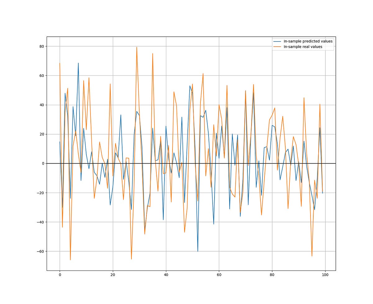
The following graph shows the in-sample predictions versus the real values. They share a strong positive correlation. The hit ratio is 63.11%.
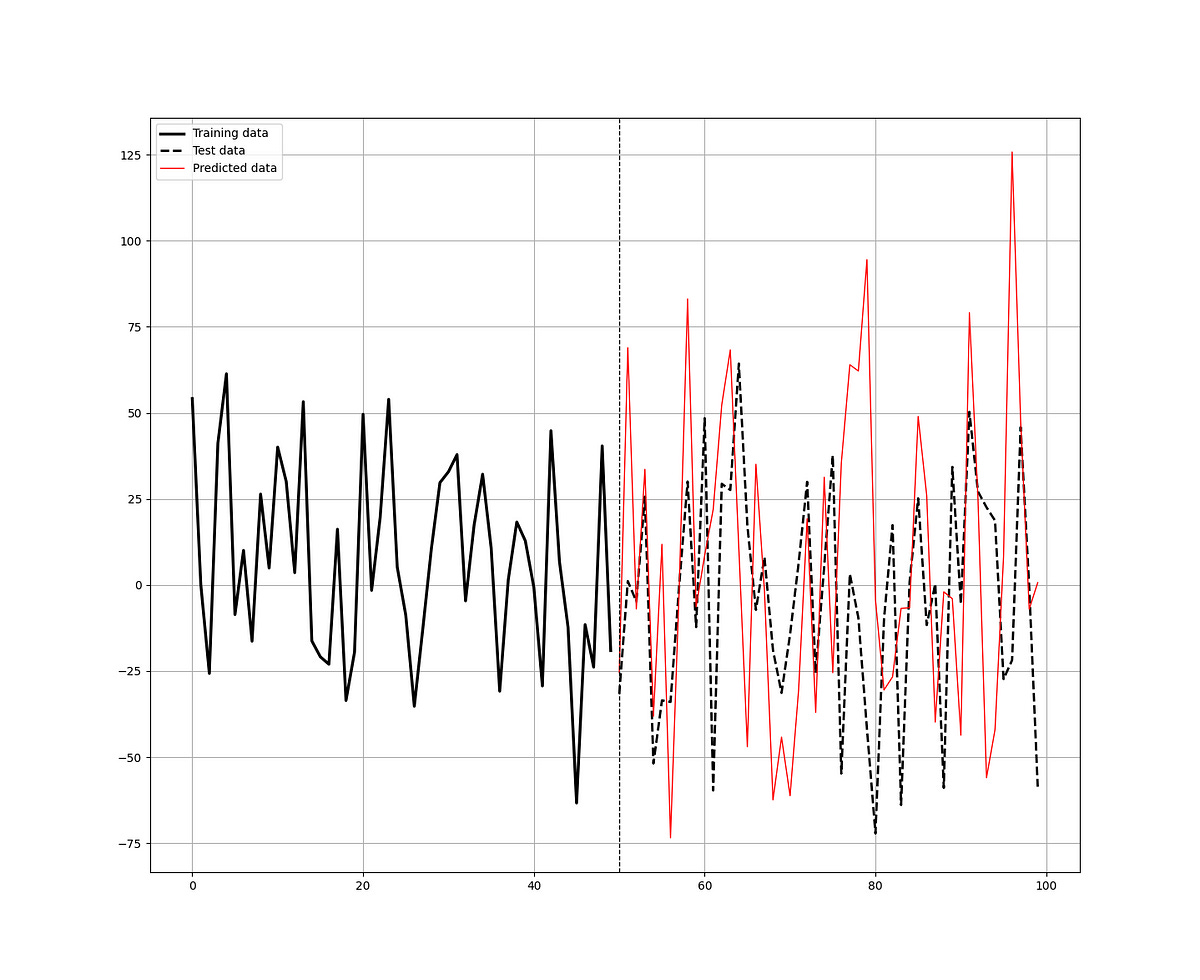
The following graph shows the in-sample predictions versus the real values. They share a weak positive correlation. The hit ratio is 55.0%.
With 2484 training data and 100 test data, the 55.0% hit ratio, and a model bias of 1.08, it seems that the model’s performance is above average with room to improvement. It may be interesting to toy around with the parameters of the model.
To sum up, while linear regression aims to find the best-fitting line without considering the complexity of the model, ridge regression adds a penalty for large coefficients, making it more conservative and less prone to overfitting. It’s a handy tool when dealing with datasets where multicollinearity or overfitting might be a concern.
You can also check out my other newsletter The Weekly Market Sentiment Report that sends tactical directional views every weekend to highlight the important trading opportunities using a mix between sentiment analysis (COT reports, Put-Call ratio, Gamma exposure index, etc.) and technical analysis.


