Learn the Difference Between Machine Learning and Deep Learning
What is Machine Learning, and for that Matter, What is Deep Learning?
Machine learning and deep learning are related terms and have overlapping concepts. This article sheds some light on the main differences between the two in the context of time series analysis.
Machine Learning With Examples
Machine learning is like teaching a computer to learn from examples. Imagine you’re teaching a kid how to recognize animals. You show them pictures of dogs, cats, and elephants, and tell them what each animal is. After seeing many examples, the kid starts to figure out the differences between them. Similarly, in machine learning, instead of a kid, you have a computer program, and instead of animals, you might have data like pictures, text, or numbers.
There are different types of machine learning, but let’s focus on the most common one: supervised learning. In supervised learning, you have a bunch of examples called training data that have inputs and corresponding outputs. For instance, if you’re trying to teach a computer to recognize handwritten digits, the inputs would be images of digits (like the number 3) and the outputs would be the labels (saying it’s a 3).
The computer then tries to find patterns in the data on its own. It might notice that certain shapes or patterns often correspond to certain labels. Once it learns these patterns from the training data, you can give it new, unseen data (like a new handwritten digit) and it can make predictions about what the correct label might be.
Now, the learning part is where the magic happens. The computer doesn’t just memorize the training examples. Instead, it tries to generalize from them, so it can correctly classify new, unseen examples it hasn’t encountered before. It’s like if the kid you were teaching about animals could correctly identify a new animal they’ve never seen before, based on the patterns they’ve learned from previous examples.
At its core, machine learning is all about getting computers to learn from data and make decisions or predictions based on that learning. It’s a powerful tool that’s being used in all sorts of fields, from healthcare to finance to self-driving cars, and it’s only getting more important as our world becomes increasingly digital and data-driven.
Let’s talk about one of the simple machine learning algorithms, and use it to predict simple time series data.
✨ Important note
We will use Python to download a sample time series data, and apply a machine learning algorithm to predict its future values based on its past values. It’s like looking at the past patterns to determine the future observations.
Linear regression is a statistical method used to understand and model the relationship between two variables. It’s like drawing a straight line through a scatter plot of data points to represent the overall trend or pattern in the data.
You have one (or more) variable, called the independent variable, which you think influences or predicts the other variable, called the dependent variable. For example, in predicting house prices, the size of the house could be the independent variable, while the price could be the dependent variable.
Linear regression helps you find the best-fitting line through the data points by minimizing the difference between the actual data points and the predicted values on the line. The equation for a straight line is usually in the form: y = mx + b, where y is the dependent variable, x is the independent variable, m is the slope (how much y changes for each unit change in x), and b is the intercept (where the line crosses the y-axis).
So, in linear regression, you’re essentially finding the best values for m and b that minimize the error between the actual data points and the predicted values on the line. Once you have this line, you can use it to make predictions for new data points. It’s a fundamental tool in statistics and machine learning, widely used in various fields like finance, economics, and social sciences.
Let’s follow this framework:
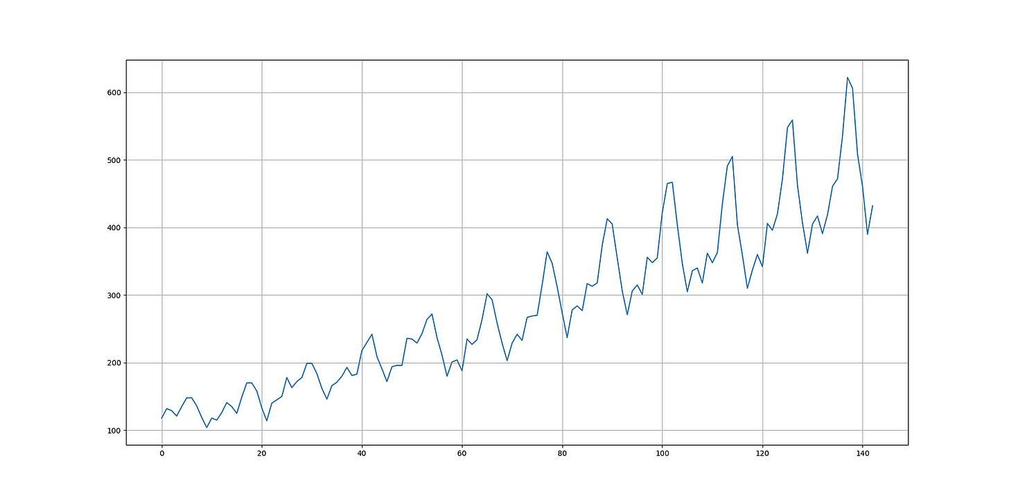
Download the air passengers time series file from here.
Define the linear regression model from sklearn library.
Make the data stationary through differencing.
Split the data into training and test sets.
Run the algorithm, and predict on the test set.
Evaluate the performance.
✨ Important note
The training set is a portion of the available data that is used to train or teach the model. Essentially, the model learns patterns, relationships, and trends from this data. It’s like giving the model examples to study so that it can understand how the independent variables relate to the dependent variable.
The test set is a separate portion of the data that the model hasn’t seen during training. It’s used to evaluate the performance of the model and to see how well it generalizes to new, unseen data. The test set helps determine if the model has learned meaningful patterns or if it’s just memorizing the training data.
Use the following code to implement the experiment:
# Importing libraries
from sklearn.linear_model import LinearRegression
import numpy as np
import matplotlib.pyplot as plt
import pandas as pd

# Fetch the CPI data
data = np.array(pd.read_excel('AirPassengers.xlsx'))
# Difference the data and make it stationary
data = np.diff(data[:, 0])
# Setting the hyperparameters
num_lags = 10
train_test_split = 0.80

def data_preprocessing(data, num_lags, train_test_split):
    # Prepare the data for training
    x = []
    y = []
    for i in range(len(data) - num_lags):
        x.append(data[i:i + num_lags])
        y.append(data[i+ num_lags])
    # Convert the data to numpy arrays
    x = np.array(x)
    y = np.array(y)
    # Split the data into training and testing sets
    split_index = int(train_test_split * len(x))
    x_train = x[:split_index]
    y_train = y[:split_index]
    x_test = x[split_index:]
    y_test = y[split_index:]

    return x_train, y_train, x_test, y_test
# Creating the training and test sets
x_train, y_train, x_test, y_test = data_preprocessing(data, num_lags, train_test_split)
model = LinearRegression()
# Train the model
model.fit(x_train, y_train)
# Predicting out-of-sample
y_pred = np.reshape(model.predict(x_test), (-1))
# Plotting
plt.plot(y_pred[-100:], label='Predicted Data', linestyle='--', marker = '.', color = 'red')
plt.plot(y_test[-100:], label='True Data', marker = '.', alpha = 0.7, color = 'blue')
plt.legend()
plt.grid()
plt.axhline(y = 0, color = 'black', linestyle = '--')
same_sign_count = np.sum(np.sign(y_pred) == np.sign(y_test)) / len(y_test) * 100
print('Hit Ratio = ', same_sign_count, '%')
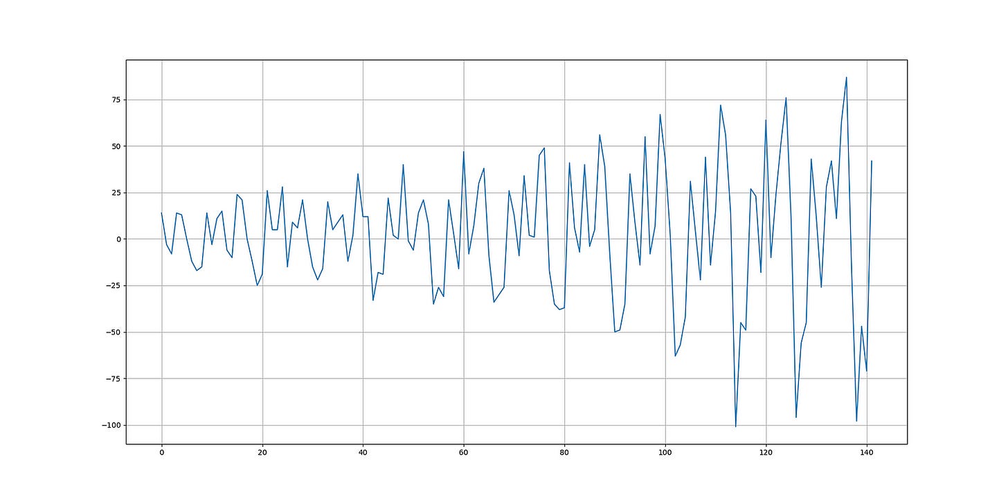
As a side note, the stationary (transformed) air passengers data looks like this:
✨ Important note
For simplicity, we will consider the data as stationary, as technically, it may or may not be since the mean and standard deviation are unlikely to be very constant. However, the transformed form of the air passenger data is more stationary than the raw (trending) form. In any case, if you want it to be more scientifically stationary, you can try differencing it one more time.
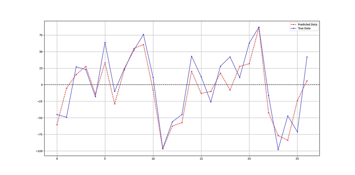
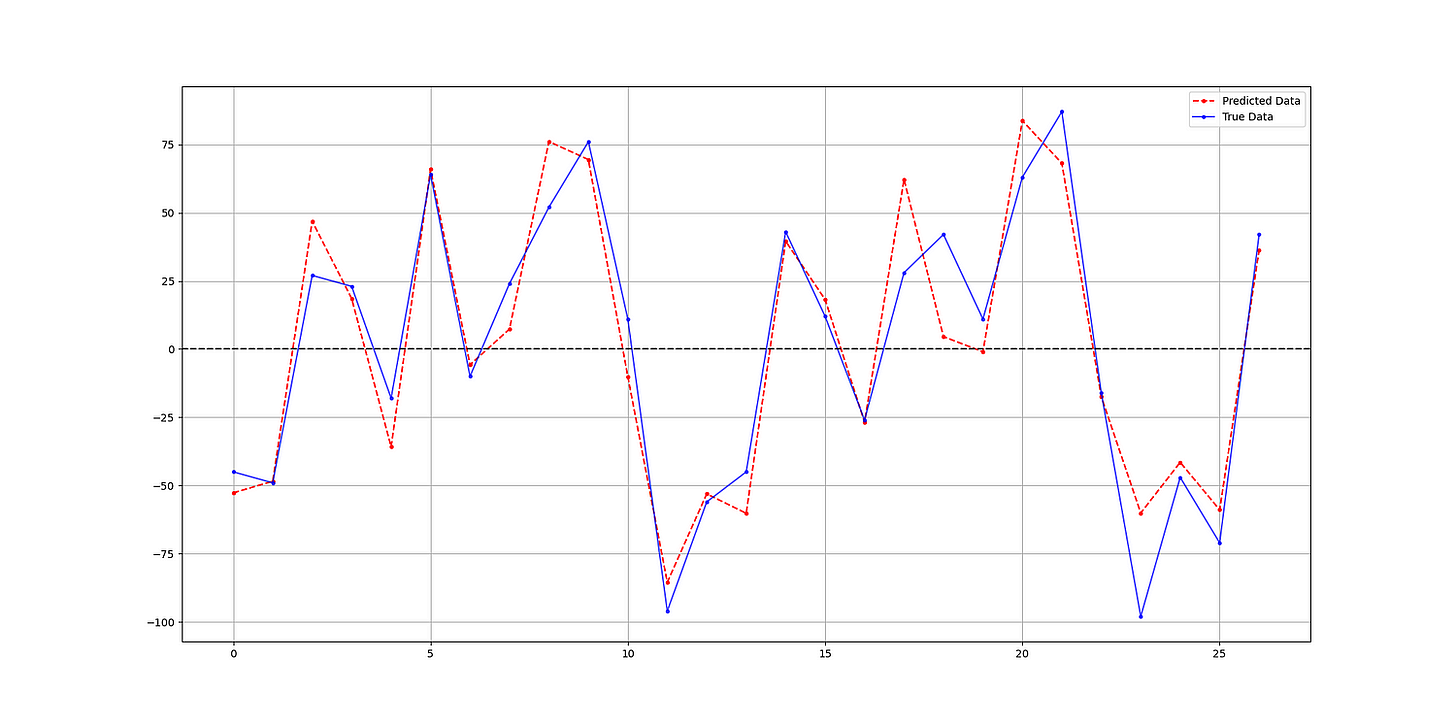
The following shows the predicted values versus the real values in the test set:
The output of the code is as follows:
Hit Ratio = 88.88888888888889 %✨ Important note
Why make the data stationary? Making the data stationary before forecasting is important because many time series forecasting techniques assume that the underlying data generating process is stationary. Stationarity refers to the statistical properties of a time series remaining constant over time.
Let’s now discover deep learning and its specificities.
If you want to see more of my work, you can visit my website for the books catalogue by simply following the link attached the picture:
Deep Learning With Examples
Deep learning is a type of machine learning that’s inspired by how the human brain works. Just like in the brain, where neurons connect to each other to process information, in deep learning, you have artificial neurons organized in layers. These layers form what’s called a neural network.
Now, what makes deep learning deep is that these neural networks have many layers stacked on top of each other. Each layer processes the data in a slightly more abstract or complex way than the previous one. For example, in an image recognition task, the first layer might look for basic features like edges or colors, while deeper layers might combine these features to recognize more complex patterns like shapes or objects.
The big advantage of deep learning is its ability to automatically learn hierarchical representations of data. Instead of having to handcraft features for the computer to look for, like in traditional machine learning, deep learning models can learn these features from the raw data itself.
Training a deep learning model involves feeding it lots of examples of inputs and their corresponding outputs, just like in other types of machine learning. But because deep learning models can have millions of parameters (the connections between neurons), training them requires a lot of data and computational power. That’s why deep learning really took off with the rise of big data and powerful GPUs (graphics processing units) that can handle all the number crunching.
One of the most famous types of deep learning architectures is the multi-layer perceptron (MLP).
The MLP algorithm is a type of artificial neural network that consists of multiple layers of interconnected nodes, or neurons. Each neuron receives input from the neurons in the previous layer, processes this information using an activation function, and passes the result to the neurons in the next layer.
In an MLP, there are typically three types of layers: input layer, hidden layers, and output layer. The input layer receives the initial data, the hidden layers perform intermediate processing, and the output layer produces the final prediction or classification.
During training, the model adjusts the weights and biases associated with each connection between neurons in order to minimize the difference between the predicted output and the actual output. This is typically done using an optimization algorithm like gradient descent.
MLPs are versatile and can be used for a wide range of tasks, including regression, classification, and pattern recognition. Let’s use it as the model for our example on the air passengers.
Use the following code to implement the experiment:
# Importing libraries
from sklearn.neural_network import MLPRegressor
import numpy as np
import matplotlib.pyplot as plt
import pandas as pd

# Fetch the CPI data
data = np.array(pd.read_excel('AirPassengers.xlsx'))
# Difference the data and make it stationary
data = np.diff(data[:, 0])
# Setting the hyperparameters
num_lags = 10
train_test_split = 0.80

def data_preprocessing(data, num_lags, train_test_split):
    # Prepare the data for training
    x = []
    y = []
    for i in range(len(data) - num_lags):
        x.append(data[i:i + num_lags])
        y.append(data[i+ num_lags])
    # Convert the data to numpy arrays
    x = np.array(x)
    y = np.array(y)
    # Split the data into training and testing sets
    split_index = int(train_test_split * len(x))
    x_train = x[:split_index]
    y_train = y[:split_index]
    x_test = x[split_index:]
    y_test = y[split_index:]

    return x_train, y_train, x_test, y_test
# Creating the training and test sets
x_train, y_train, x_test, y_test = data_preprocessing(data, num_lags, train_test_split)
model = MLPRegressor()
# Train the model
model.fit(x_train, y_train)
# Predicting out-of-sample
y_pred = np.reshape(model.predict(x_test), (-1))
# Plotting
plt.plot(y_pred[-100:], label='Predicted Data', linestyle='--', marker = '.', color = 'red')
plt.plot(y_test[-100:], label='True Data', marker = '.', alpha = 0.7, color = 'blue')
plt.legend()
plt.grid()
plt.axhline(y = 0, color = 'black', linestyle = '--')
same_sign_count = np.sum(np.sign(y_pred) == np.sign(y_test)) / len(y_test) * 100
print('Hit Ratio = ', same_sign_count, '%')
The following shows the predicted values versus the real values in the test set:
The output of the code is as follows:
Hit Ratio = 92.5925925925926 %Deep learning has been behind many breakthroughs in artificial intelligence in recent years, from speech recognition to natural language processing to autonomous vehicles. Its ability to automatically learn complex patterns from raw data has made it one of the most powerful tools in the machine learning toolbox.
The Main Differences Between Machine Learning and Deep Learning
When it comes to analyzing time series data, machine learning algorithms tend to be simpler in structure compared to deep learning models. These models often rely on handcrafted features and may struggle with capturing complex temporal patterns. Deep learning models are specifically designed to handle sequential data like time series. These models have more complex architectures with layers of interconnected neurons, allowing them to capture intricate temporal dependencies within the data.
Additionally, machine learning engineers often spend a significant amount of time manually selecting and engineering features from the time series data. These features could include statistical measures, lagged variables, or domain-specific indicators. Deep learning models for time series analysis can automatically learn relevant features from raw data, eliminating the need for extensive manual feature engineering.
Furthermore, traditional machine learning models may require a moderate amount of labeled training data to generalize well to new time series datasets. The quality and quantity of features engineered by domain experts can significantly impact the model’s performance. Deep learning models often require large amounts of labeled training data to effectively learn complex patterns from time series data. However, once trained on sufficient data, deep learning models can generalize well to new datasets and exhibit strong predictive capabilities.
Lastly, traditional machine learning models are often more interpretable, as the relationship between input features and output predictions is more transparent. Engineers can analyze feature importance and model coefficients to understand how the model makes predictions. Deep learning models, particularly those with complex architectures may sacrifice interpretability for predictive performance. Understanding how individual neurons in deep neural networks contribute to predictions can be challenging, making these models less transparent.
While both machine learning and deep learning can be applied to time series analysis, deep learning models offer advantages in automatically learning complex temporal patterns from raw data without extensive feature engineering. However, deep learning models may require larger datasets and computational resources, and they may be less interpretable compared to traditional machine learning models.
You can also check out my other newsletter The Weekly Market Sentiment Report that sends tactical directional views every weekend to highlight the important trading opportunities using a mix between sentiment analysis (COT reports, Put-Call ratio, Gamma exposure index, etc.) and technical analysis.


