Identifying Momentum Reversals With Extreme Duration
Creating & Coding the Extreme Duration to Trade the Markets
In technical analysis, we spend time analyzing when markets are oversold and overbought but we never look at how long do they stay oversold and overbought. What if the duration of time spent oversold/overbought can help us know when on average, the market will finally react? Most of the time, we are happy to see that we are on extremes with regards to a technical indicator, only to realize that the extreme condition could last ages without the market reacting.
This is the beauty of randomness and the enormous amount of buyers/sellers for different reasons. In this article, we will create the function that lets us calculate the time spent around the extremes and analyze the signals generated by entering upon a specific timing.
The Relative Strength Index
First introduced by J. Welles Wilder Jr., the RSI is one of the most popular and versatile technical indicators. Mainly used as a contrarian indicator where extreme values signal a reaction that can be exploited. Typically, we use the following steps to calculate the default RSI:
Calculate the change in the closing prices from the previous ones.
Separate the positive net changes from the negative net changes.
Calculate a smoothed moving average on the positive net changes and on the absolute values of the negative net changes.
Divide the smoothed positive changes by the smoothed negative changes. We will refer to this calculation as the Relative Strength — RS.
Apply the normalization formula shown below for every time step to get the RSI.
The above chart shows the hourly values of the GBPUSD in black with the 13-period RSI. We can generally note that the RSI tends to bounce close to 25 while it tends to pause around 75. To code the RSI in Python, we need an OHLC array composed of four columns that cover open, high, low, and close prices.
def adder(data, times):

    for i in range(1, times + 1):

        new = np.zeros((len(data), 1), dtype = float)

        data = np.append(data, new, axis = 1)
return datadef deleter(data, index, times):
for i in range(1, times + 1):
data = np.delete(data, index, axis = 1)return data
def jump(data, jump):
data = data[jump:, ]
return datadef ma(data, lookback, close, where):
data = adder(data, 1)
for i in range(len(data)):
try:
data[i, where] = (data[i - lookback + 1:i + 1, close].mean())
except IndexError:
pass
data = jump(data, lookback)
return datadef ema(data, alpha, lookback, what, where):
alpha = alpha / (lookback + 1.0)
beta = 1 - alpha
data = ma(data, lookback, what, where)data[lookback + 1, where] = (data[lookback + 1, what] * alpha) + (data[lookback, where] * beta)for i in range(lookback + 2, len(data)):
try:
data[i, where] = (data[i, what] * alpha) + (data[i - 1, where] * beta)
except IndexError:
pass
return datadef rsi(data, lookback, close, where):
data = adder(data, 5)
for i in range(len(data)):
data[i, where] = data[i, close] - data[i - 1, close]
for i in range(len(data)):
if data[i, where] > 0:
data[i, where + 1] = data[i, where]
elif data[i, where] < 0:
data[i, where + 2] = abs(data[i, where])
lookback = (lookback * 2) - 1 # From exponential to smoothed
data = ema(data, 2, lookback, where + 1, where + 3)
data = ema(data, 2, lookback, where + 2, where + 4) data[:, where + 5] = data[:, where + 3] / data[:, where + 4]
data[:, where + 6] = (100 - (100 / (1 + data[:, where + 5]))) data = deleter(data, where, 6)
data = jump(data, lookback)return dataKnowledge must be accessible to everyone. This is why, from now on, a purchase of either one of my new books “Contrarian Trading Strategies in Python” or “Trend Following Strategies in Python” comes with free PDF copies of my first three books (Therefore, purchasing one of the new books gets you 4 books in total). The two new books listed above feature a lot of advanced indicators and strategies with a GitHub page. You can use the below link to purchase one of the two books (Please specify which one and make sure to include your e-mail in the note).
Pay Kaabar using PayPal.Me
Go to paypal.me/sofienkaabar and type in the amount. Since it’s PayPal, it’s easy and secure. Don’t have a PayPal…www.paypal.com
The Extreme Duration
I have presented the RSI first because the extreme duration is simply an add-on to any bounded indicator. It is not an indicator on its own per se, but simply a way to see how long the indicator spends being overbought or oversold. We understand that:
An overbought indicator is saying that the bullish momentum should fade soon and we might see a correction or even a reversal on the downside.
An oversold indicator is saying that the bearish momentum should fade soon and we might see a correction or even a reversal on the upside.
However, if things were so simple, we would all be millionaires. With this being said, let us take a look at the extreme duration below (calculated on the values of the RSI) before seeing how to code and analyze it.
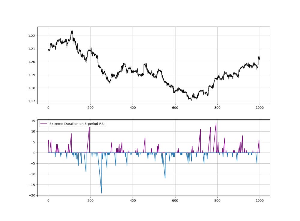
The above plot shows the extreme duration calculation based on a 5-period RSI with barriers at 70 and 30. When the Extreme Duration is showing a reading of 5, it means that the 5-period RSI is above 70 for the fifth consecutive time (i.e. surpassed 70 and stayed above it for 5 units of time). We are used to analyze these indicators value-wise, we want to analyze them this time time-wise. To calculate the extreme duration, we can follow the below steps:
# Calculate the RSI on OHLC array (composed of 4 columns)
my_data = rsi(my_data, 5, 3, 4)
# Define the Barriers (Oversold and Overbought zones)
upper_barrier = 70
lower_barrier = 30# Define the Extreme Duration
def extreme_duration(data, indicator, upper_barrier, lower_barrier, where_upward_extreme, where_downward_extreme):
data = adder(data, 2)# Time Spent Overbought
for i in range(len(data)):
if data[i, indicator] > upper_barrier:
data[i, where_upward_extreme] = data[i - 1, where_upward_extreme] + 1
else:
a = 0
data[i, where_upward_extreme] = a
# Time Spent Oversold
for i in range(len(data)):
if data[i, indicator] < lower_barrier:
data[i, where_downward_extreme] = data[i - 1, where_downward_extreme] + 1
else:
a = 0
data[i, where_downward_extreme] = a
data[:, where_downward_extreme] = -1 * data[:, where_downward_extreme]
return data# Calculating the Extreme Duration
my_data= extreme_duration(my_data, 4, upper_barrier, lower_barrier, 5, 6)Let us now try to use the extreme duration to generate signals based on this hypothesis:
“What if the average time spent on the extremes can help us understand when the indicator will exist these mentioned extremes?”
Based on a historical analysis, the average duration of the 5-period RSI is between 3 and 4. However, based on visual historical representation, it is closer to 5. Let us set the time barriers to 5 and -5.
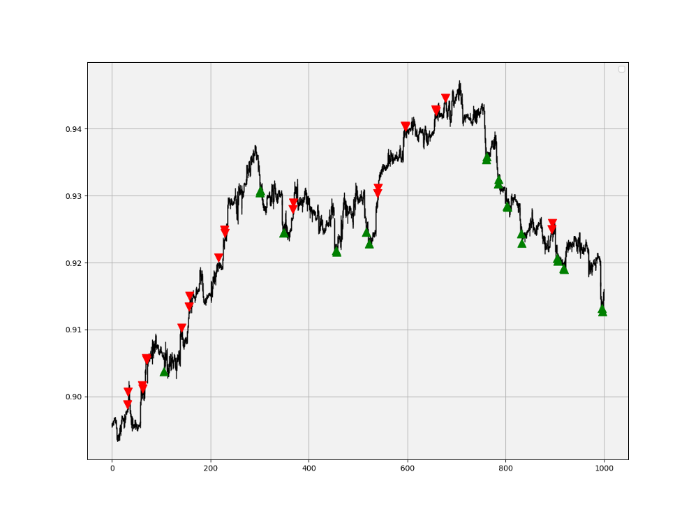
The above plot shows the signals generated when the 5-period RSI on the EURUSD hourly data remains for at least 5 periods on the extremes.
def signal(data, upward_timing, downward_timing, buy, sell):data = adder(data, 2)for i in range(len(data)):
if data[i, downward_timing] <= -5 and data[i - 1, downward_timing] >= -5 and data[i - 2, downward_timing] >= -5:
data[i, buy] = 1
if data[i, upward_timing] >= 5 and data[i - 1, upward_timing] <= 5 and data[i - 2, upward_timing] <= 5 :
data[i, sell] = -1
return dataA lot of optimization can be done on this promising technique, especially that only value-wise readings are not sufficient anymore. Temporal analysis is paramount to better understand how the underlying reacts.
If you want to see how to create all sorts of algorithms yourself, feel free to check out Lumiwealth. From algorithmic trading to blockchain and machine learning, they have hands-on detailed courses that I highly recommend.
Learn Algorithmic Trading with Python Lumiwealth
Learn how to create your own trading algorithms for stocks, options, crypto and more from the experts at Lumiwealth. Click to learn more
Summary
To sum up, what I am trying to do is to simply contribute to the world of objective technical analysis which is promoting more transparent techniques and strategies that need to be back-tested before being implemented. This way, technical analysis will get rid of the bad reputation of being subjective and scientifically unfounded.
I recommend you always follow the the below steps whenever you come across a trading technique or strategy:
Have a critical mindset and get rid of any emotions.
Back-test it using real life simulation and conditions.
If you find potential, try optimizing it and running a forward test.
Always include transaction costs and any slippage simulation in your tests.
Always include risk management and position sizing in your tests.
Finally, even after making sure of the above, stay careful and monitor the strategy because market dynamics may shift and make the strategy unprofitable.


