
I Backtested a Powerful Strategy on Bitcoin - The Results
Let's See What the Results From This Strategy Say


Every indicator promises an edge — until the market reminds you that edges can dull fast. I set out to backtest a Bitcoin strategy that combines two of the most time-tested tools in technical analysis: moving averages and the RSI.
The goal is simple — identify moments when short-term momentum aligns with longer-term trend structure, and test if that alignment could reliably capture the big swings.
The results were... surprising. What looked like a textbook setup on paper turned out to behave very differently once we let the data tell the story.
Introduction to the Components of the Strategy
Markets are noisy. Price jerks up and down, candles flicker, and it’s easy to lose the plot. A moving average doesn’t try to predict anything. It just tells you where the center of gravity has been, over a chosen window of time.
The most basic version is the average price over the last n periods:
If you plot it, it smooths the price line, filtering out minor fluctuations. A 50-day SMA gives you the average closing price of the last 50 days. A 200-day SMA? That’s the long view, often used to judge whether an asset is in a bull or bear phase.
If moving averages tell you the direction, the Relative Strength Index (RSI) tells you the intensity—the momentum. It’s an oscillator that measures how strongly price has moved up or down over the last 14 periods (by default). It gives you a number between 0 and 100.
Here’s the basic formula:
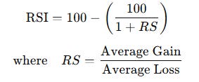
So if the average gain is way higher than the average loss, RSI rises. If losses dominate, it drops. And the number you get isn’t abstract—it’s readable:
RSI > 70: Market is considered overbought. May be due for a pullback.
RSI < 30: Market is oversold. Could be ready to bounce.
But here’s the nuance: RSI doesn’t say “sell at 70” or “buy at 30.” In strong trends, RSI can stay above 70 for days or weeks. Overbought doesn’t mean bearish—it means strong. Similarly, oversold doesn’t guarantee a reversal—it means weak.
The Signal Beyond 🚀.
From classic tools that have stood the test of time to fresh innovations like multi-market RSI heatmaps, COT reports, seasonality, and pairs trading recommendation system, the new report is designed to give you a sharper edge in navigating the markets.
Free trial available.
Creating and Back-testing the Strategy in Python
The strategy is quite simple really:
A bullish trade is generated whenever the current short-term SMA is above the current long-term SMA and the previous RSI is below the oversold level and below the current RSI.
A bearish trade is generated whenever the current short-term SMA is below the current long-term SMA and the previous RSI is above the overbought level and above the current RSI.
We will tweak the following parameters and back-test on the daily values of BTCUSD:
short_len = this is the lookback period of the short SMA
long_len = this is the lookback period of the long SMA
rsi_ov = this is the overbought level
rsi_us = this is the oversold level
initial_capital = this is the initial balance
holding_period = this is the number of periods to hold before liquidating
We will try three different variations of the strategy:
A long-only strategy
A short-only strategy
A strategy that combines both signals (long and short)
Let’s see what the results were.
It is extremely important to read the next section after you look at the back-testing results.
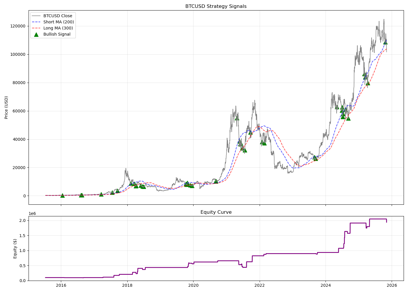
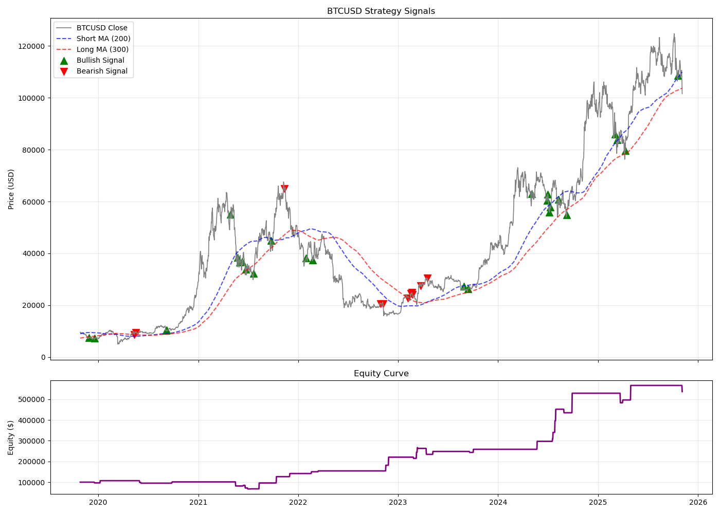
The parameters of the only-Bull strategy are as follows:
short_len = 200
long_len = 300
rsi_ov = 60
rsi_us = 35
initial_capital = 100000
holding_period = 20
The following shows the signals and the equity curve throughout the years.
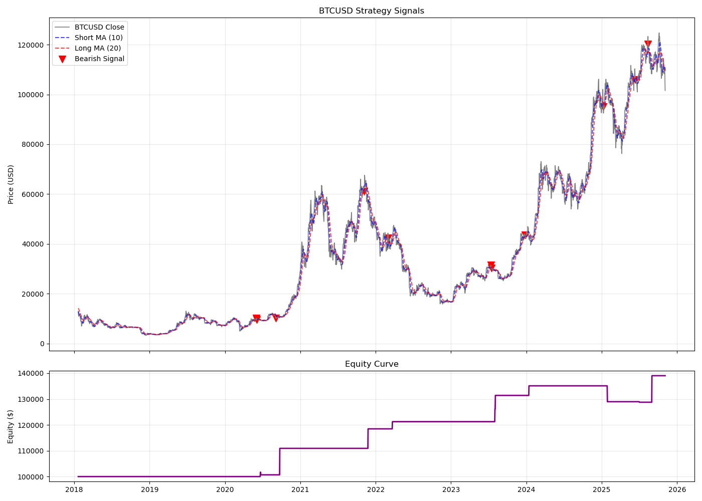
The parameters of the only-Bear strategy are as follows:
short_len = 10
long_len = 20
rsi_ov = 60
rsi_us = 30
initial_capital = 100000
holding_period = 20
The following shows the signals and the equity curve throughout the years.
The parameters of the Bull-Bear strategy are as follows:
short_len = 200
long_len = 300
rsi_ov = 65
rsi_us = 35
initial_capital = 100000
holding_period = 20
The following shows the signals and the equity curve throughout the years.
Use the following code to implement the Bull-Bear experimentation:
import yfinance as yf
import numpy as np
import matplotlib.pyplot as plt
import pandas as pd


# --- Parameters ---
short_len = 200
long_len = 300
rsi_ov = 65
rsi_us = 35
initial_capital = 100000
holding_period = 20
# --- Download Data ---
data = yf.download(”BTC-USD”, start=”2019-01-01”, end=”2025-11-07”)

# --- Indicators ---
data[’SMA_short’] = data[’Close’].rolling(short_len).mean()
data[’SMA_long’] = data[’Close’].rolling(long_len).mean()

def rsi(my_time_series, source=’close’, output_name=’RSI’, rsi_lookback=14):
    # calculating the difference between the close prices at each time step
    delta = my_time_series[source].diff(1)
    # isolating the positive differences and the absolute negative differences
    gain = delta.where(delta > 0, 0)
    loss = -delta.where(delta < 0, 0)
    # transforming the exponential moving average to a smoothed moving average
    rsi_real_lookback = (rsi_lookback*2)-1
    # calculating a rolling smoothed moving average on the gain and loss variables
    avg_gain = gain.ewm(span=rsi_real_lookback, min_periods=1, adjust=False).mean()
    avg_loss = loss.ewm(span=rsi_real_lookback, min_periods=1, adjust=False).mean()
    # calculating the relative strength
    rs = avg_gain / avg_loss
    # calculating the relative strength index
    rsi = 100-(100/(1+rs))
    # creating a column in the data frame and populating it with the RSI
    my_time_series[output_name] = rsi
    return my_time_series.dropna()

data = rsi(data, source=’Close’, output_name=’RSI’, rsi_lookback=14)
data.columns = data.columns.get_level_values(0)

# --- Signal Columns ---
data[’bullish_entry’] = 0
data[’bearish_entry’] = 0

# --- Detect Bullish/Bearish Confirmations ---
for i in range(1, len(data)-1):
    if data[’SMA_short’].iloc[i] > data[’SMA_long’].iloc[i] and data[’RSI’].iloc[i-1] < rsi_us <= data[’RSI’].iloc[i]:
        data.at[data.index[i+1], ‘bullish_entry’] = 1
    elif data[’SMA_short’].iloc[i] < data[’SMA_long’].iloc[i] and data[’RSI’].iloc[i-1] > rsi_ov >= data[’RSI’].iloc[i]:
        data.at[data.index[i+1], ‘bearish_entry’] = 1

# --- Simulate Trades & Equity Curve (in sync with data) ---
data[’Trade_Profit’] = 0.0
equity = initial_capital

for i in range(len(data)):
    if data[’bullish_entry’].iloc[i] == 1:
        entry_price = data[’Open’].iloc[i]
        exit_idx = min(i + holding_period, len(data) - 1)
        exit_price = data[’Close’].iloc[exit_idx]
        profit = (exit_price - entry_price) / entry_price
        data.loc[data.index[exit_idx], ‘Trade_Profit’] += profit
    elif data[’bearish_entry’].iloc[i] == 1:
        entry_price = data[’Open’].iloc[i]
        exit_idx = min(i + holding_period, len(data) - 1)
        exit_price = data[’Close’].iloc[exit_idx]
        profit = (entry_price - exit_price) / entry_price
        data.loc[data.index[exit_idx], ‘Trade_Profit’] += profit

# --- Compute Cumulative Profit (Equity Curve) ---
data[’CumProfit’] = (1 + data[’Trade_Profit’]).cumprod() * initial_capital

# --- Plot BTCUSD + Signals and Equity Curve ---
fig, axes = plt.subplots(2, 1, figsize=(14, 10), sharex=True, gridspec_kw={’height_ratios’: [3, 1]})

# Price Chart
axes[0].plot(data[’Close’], label=’BTCUSD Close’, color=’gray’, linewidth=1.2)
axes[0].plot(data[’SMA_short’], label=f’Short MA ({short_len})’, color=’blue’, linestyle=’--’, alpha=0.7)
axes[0].plot(data[’SMA_long’], label=f’Long MA ({long_len})’, color=’red’, linestyle=’--’, alpha=0.7)
axes[0].scatter(data.index[data[’bullish_entry’] == 1], data[’Close’][data[’bullish_entry’] == 1],
                marker=’^’, color=’green’, s=100, label=’Bullish Signal’)
axes[0].scatter(data.index[data[’bearish_entry’] == 1], data[’Close’][data[’bearish_entry’] == 1],
                marker=’v’, color=’red’, s=100, label=’Bearish Signal’)
axes[0].set_title(’BTCUSD Strategy Signals’)
axes[0].set_ylabel(’Price (USD)’)
axes[0].legend()
axes[0].grid(alpha=0.3)

# Equity Curve
axes[1].plot(data[’CumProfit’], color=’purple’, linewidth=2)
axes[1].set_title(’Equity Curve’)
axes[1].set_ylabel(’Equity ($)’)
axes[1].grid(alpha=0.3)

plt.tight_layout()
plt.show()

# --- Performance Summary ---
num_trades = (data[’Trade_Profit’] != 0).sum()
wins = (data[’Trade_Profit’] > 0).sum()
hit_ratio = wins / num_trades if num_trades > 0 else np.nan
gains = data.loc[data[’Trade_Profit’] > 0, ‘Trade_Profit’].sum()
losses = -data.loc[data[’Trade_Profit’] < 0, ‘Trade_Profit’].sum()
profit_factor = gains / losses if losses != 0 else np.nan

print(f”\nNumber of trades: {num_trades}”)
print(f”Hit ratio: {hit_ratio:.2%}”)
print(f”Profit factor: {profit_factor:.2f}”)
print(f”Final equity: ${data[’CumProfit’].iloc[-1]:,.2f}”)
The Mirage of Backtesting: Why Profitable Strategies Often Aren’t
Backtesting is a powerful microscope — it lets us see what might have worked. But too often, traders mistake that microscope for a crystal ball.
A backtest is not the market; it’s a simulation stitched together with assumptions, biases, and simplifications that may collapse under real-world uncertainty.
The Problem of Selective Optimization
Most backtests begin with a seemingly innocent question: “What parameters work best?”
But the moment you start adjusting moving average lengths, RSI thresholds, or holding periods to improve historical performance, you enter the domain of data-mining bias.
You’re no longer testing a universal principle — you’re optimizing noise.
Every tweak that improves your equity curve is a trade-off: you gain in-sample precision but lose out-of-sample robustness.
In other words:
You didn’t find a strategy that works; you found the one that fits yesterday’s noise perfectly.
And the market, being a living organism of uncertainty, changes structure faster than your backtest adapts.
Low Trade Frequency = Statistical Mirage
One of the most seductive metrics in backtesting is the profit factor — the ratio of total gains to total losses.
A high profit factor (say, 2.0 or above) often makes traders feel like they’ve found an edge. But in low-frequency systems — say, strategies that trigger only 20–30 trades over several years — the math is deceptive.
If you only have 25 trades:
One or two lucky trades can double your profit factor.
A single outlier loss can wipe it out.
In statistical terms, the sample size is too small to draw any inference about expected value. The variance of outcomes is so high that you’re effectively flipping a coin and pretending you discovered a law of physics.
When the number of observations is low, randomness dominates. In a 10-year backtest with 20 trades, you don’t have a “strategy” — you have a sequence of anecdotes.
The Hidden Bias: Bullish Strategies in Bullish Markets
Bitcoin — and many other assets over long horizons — have a persistent upward drift.
This means that any strategy biased toward long trades (buy signals) will appear profitable, not because of superior logic, but because the underlying asset rose over time.
This is the bullish drift bias:
Buy-and-hold Bitcoin from 2015–2021, and you’ll “outperform” 99% of strategies.
A moving-average crossover strategy that mostly goes long will seem brilliant — but it’s just riding the secular uptrend.
Even if your rules are random, a predominance of long trades in an uptrend yields “positive” performance.
To truly test robustness, you need to stress-test the same logic in:
Bear markets
Sideways consolidations
Different assets (non-correlated markets)
Forward periods never seen by the model
If your “edge” disappears when the environment changes, you never had an edge — you had a regime dependency disguised as skill.
Overconfidence in Historical Consistency
Humans love smooth equity curves. We see a backtest that grows steadily, and our brain interprets that as proof of predictability.
But those smooth lines often result from lookahead bias (using future data unintentionally), survivorship bias (ignoring delisted assets), or incorrect execution assumptions (like assuming you can enter at the next bar’s open with no slippage).
In reality:
Slippage, liquidity, and transaction costs can turn theoretical profits into real losses.
Execution delays or API errors in live conditions don’t exist in backtests.
Correlations between indicators (e.g., RSI and moving averages) create redundant confirmation — the illusion of robust convergence when both are reacting to the same lagging input.
The Need for Statistical Significance
Any serious evaluation of a trading strategy must ask:
How many independent trades are in the sample?
What is the t-statistic or Sharpe ratio of the returns?
Is the result consistent across time segments and assets?
Without those, your “edge” is indistinguishable from randomness.
A backtest that shows a 2.0 profit factor over 20 trades tells you almost nothing.
A backtest that shows a 1.2 profit factor over 2,000 trades tells you something.
The first is a coincidence; the second is a pattern.
Out-of-Sample and Forward Testing
True robustness comes when you deliberately withhold part of your data (out-of-sample testing) or run your system forward in live conditions (paper trading).
If the logic holds when exposed to unseen data, that’s the beginning of validity.
If not, you’ve just built a beautiful story on quicksand.
A backtest is a map of what might have happened — not the territory of what will.
Markets evolve, correlations break, regimes shift, and liquidity vanishes just when you need it most.
Any backtest that doesn’t incorporate this uncertainty is a fragile dream.
So when you see a high profit factor, a perfect equity curve, or a system that “only trades a few times a year but never loses” — remember:
It’s not proof of skill. It’s proof of selective storytelling.
Backtesting isn’t about predicting the future; it’s about estimating how wrong you could be — and surviving when you inevitably are.
Do you want to master Deep Learning techniques tailored for time series, trading, and market analysis🔥? My book breaks it all down from basic machine learning to complex multi-period LSTM forecasting while going through concepts such as fractional differentiation and forecasting thresholds. Get your copy here 📖!