How to Create Seasonal Market Charts Using Python
Creating Seasonal Charts to Look For Patterns in Equity Markets
Seasonal charts, also known as seasonal patterns or seasonal analysis, are graphical representations of historical price or performance trends of a particular asset, such as a stock, commodity, currency, or market index, over a specific time period.
These charts are used by traders, investors, and analysts to identify recurring patterns and trends that tend to occur during certain times of the year or at specific intervals. This article will show how to create a seasonality chart on the S&P 500 and how to interpret it.
Seasonality and Patterns in Financial Markets
Seasonal charts focus on analyzing price or performance data over different seasons, months, or weeks within a year. This analysis is based on the idea that certain assets or markets exhibit repetitive patterns or behaviors during particular times of the year.
To create a seasonal chart, historical price or performance data for an asset is collected and organized by time periods (e.g., months or quarters) over multiple years. This data is then averaged or otherwise adjusted to create a clear visual representation of seasonal trends. Seasonal charts typically take the form of line graphs. The x-axis represents time (e.g., days), while the y-axis represents the average price or performance of the asset. Each point on the chart corresponds to the average price or performance during a specific time period.
By studying seasonal charts, analysts look for recurring patterns and trends. For example, in the stock market, certain stocks may exhibit a pattern of rising prices during the holiday season due to increased consumer spending. Seasonal charts can be used as a tool to support trading and investment decisions. Traders may use them to identify potential entry or exit points based on historical trends, while investors may use them to allocate assets more effectively throughout the year.
While seasonal charts can provide valuable insights, it’s essential to recognize that past performance is not indicative of future results. Seasonal patterns can change over time due to various factors, including economic conditions, geopolitical events, and shifts in market sentiment. Therefore, it’s important to use seasonal analysis as one of several tools in a comprehensive investment or trading strategy. Some industries or assets are more prone to seasonal patterns than others. For example, agricultural commodities like wheat and corn often exhibit strong seasonal patterns due to planting and harvesting seasons, while technology stocks may have different seasonal influences.
Creating a Seasonal Chart on the S&P 500 Index and the Russell 2000 in Python
Creating a seasonality chart is simple in Python. You just have to find a way to average the days of the year across the different time axes.
The full code to create the seasonal chart is as follows (remember to call the function with the right market name from yahoo finance (^GSPC for the S&P 500 index and ^RUT for the Russell 2000 index)
import yfinance as yf # Make sure to pip install this
import pandas as pd
import numpy as np
import matplotlib.pyplot as plt

def seasonality_chart(market):
    start_date = "1990-01-01"
    end_date   = "2022-12-31"

    sp500_data = yf.download(market, start = start_date, end = end_date)
    sp500_data['Return'] = sp500_data['Close'].pct_change()
    sp500_data['Year'] = sp500_data.index.year
    sp500_data['DayOfYear'] = sp500_data.index.dayofyear
    average_sp500_by_day = sp500_data.groupby(['DayOfYear', 'Year'])['Return'].mean().reset_index()
    overall_average_sp500 = average_sp500_by_day.groupby('DayOfYear')['Return'].mean().reset_index()
    overall_average_sp500['Cumulative Return'] = (1 + overall_average_sp500['Return']).cumprod()

    start_date = "2023-01-01"
    end_date   = "2023-12-31"

    sp500_data_current_year = yf.download(market, start = start_date, end = end_date)
    sp500_data_current_year['Return'] = sp500_data_current_year['Close'].pct_change()
    sp500_data_current_year['Year'] = sp500_data_current_year.index.year
    sp500_data_current_year['DayOfYear'] = sp500_data_current_year.index.dayofyear
    average_sp500_by_day_current_year = sp500_data_current_year.groupby(['DayOfYear', 'Year'])['Return'].median().reset_index()
    overall_average_sp500_current_year = average_sp500_by_day_current_year.groupby('DayOfYear')['Return'].median().reset_index()
    overall_average_sp500_current_year['Cumulative Return'] = (1 + overall_average_sp500_current_year['Return']).cumprod()

    # Plot the average S&P 500 values by day of the year
    plt.plot(overall_average_sp500['DayOfYear'], overall_average_sp500['Cumulative Return'], color = 'blue', label = 'Seasonality')
    plt.plot(overall_average_sp500_current_year['DayOfYear'], overall_average_sp500_current_year['Cumulative Return'], color = 'black', label = 'Current Year')
    plt.xlabel('Day of the Year')
    plt.grid()
    plt.show()
    plt.legend()

    return overall_average_sp500, overall_average_sp500_current_year

# Calling the function
overall_average_sp500, overall_average_sp500_current_year = seasonality_chart('^RUT')
combination = pd.concat([overall_average_sp500.iloc[:len(overall_average_sp500_current_year)]['Cumulative Return'],
                         overall_average_sp500_current_year['Cumulative Return']], axis = 1)
combination = combination.iloc[1:]
combination.columns = ['First', 'Second']
correlation = combination['First'].corr(combination['Second'])
The following chart shows the seasonality on S&P 500, the main equity index in the US. Notice how approaximately, in 2023, the market followed the seasonality time series, and is now supposed to shape a bottom which will make it continue the bull trend until the end of the year.
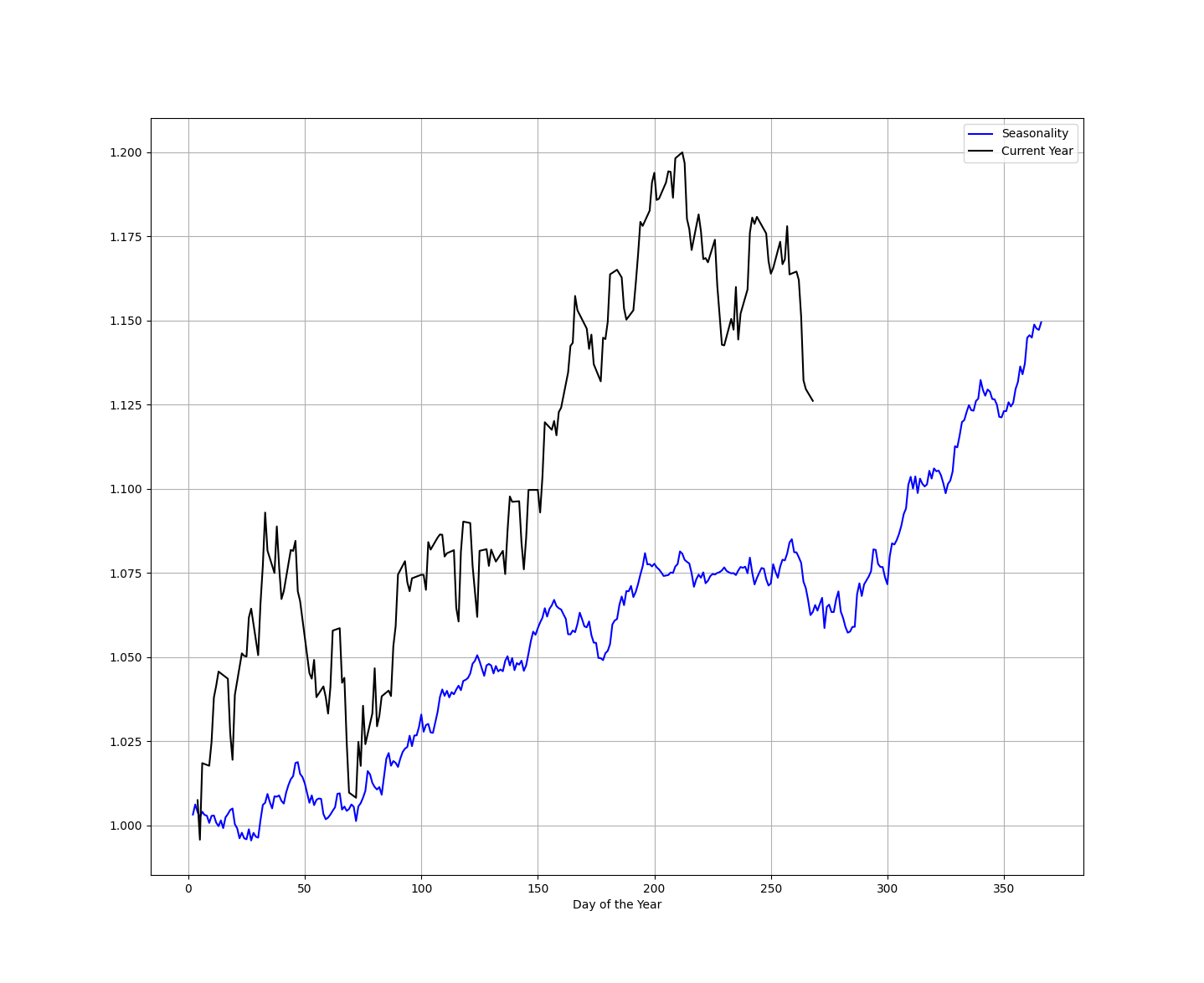
The following chart shows the seasonality on Russell 2000, another equity index in the US. It seems to also suggest that the market is approaching a bottom and is set for a rally towards the end of the year.
Bear in mind that these seasonality charts are not meant to have predictive power. Their analysis is interesting, but in no way should they be used to forecast the markets with conviction.
In summary, seasonal charts are a visual representation of historical price or performance patterns of assets over specific time intervals. They can be useful for identifying potential trading or investment opportunities, but they should be used in conjunction with other forms of analysis and with an awareness of the limitations of historical data in predicting future market behavior.
You can also check out my other newsletter The Weekly Market Sentiment Report that sends weekly directional views every weekend to highlight the important trading opportunities using a mix between sentiment analysis (COT report, put-call ratio, etc.) and rules-based technical analysis.
If you liked this article, do not hesitate to like and comment, to further the discussion!


