How Good is Stochastic Gradient Descent in Predicting Time Series?

Step-by-Step Guide to Create the SGD Machine Learning Model

Continuing with our quest to master simple and complex machine learning time series models, in this article, we’ll delve into how stochastic gradient descent (SGD) works and how it can be leveraged to make predictions.

Stochastic Gradient Descent

SGD regression is a powerful optimization technique used for training machine learning models, particularly linear regression models. Unlike traditional gradient descent (GD), which computes the gradient of the cost function using the entire dataset, SGD updates the model parameters after evaluating a single data point or a small batch.

This makes it much more efficient in terms of memory and computation, especially when working with large datasets.

At its core, SGD is an iterative optimization algorithm that aims to minimize a loss function by updating the parameters (e.g., weights) of the model in the opposite direction of the gradient.

This process gradually reduces the difference between the predicted values and the true values (minimizing the error). The steps involved in SGD regression are as follows:

1. Start with initial guesses for the parameters (weights and bias). These are typically set randomly or to zero.

2. For each iteration, randomly select a single data point (or a small batch in mini-batch SGD) from the dataset.

3. Compute the gradient of the loss function with respect to the model parameters. In the case of linear regression, the mean squared error (MSE) is typically used as the loss function. The gradient is calculated as:

• Once the gradient is calculated, the model parameters arre updated in the opposite direction of the gradient:

• Repeat the process for a set number of iterations or until the model parameters converge, meaning the change in the loss function is minimal.

Let’s see how to use this model for time series analysis (inflation data).

Creating the Model

Let’s create the model in Python by importing data and the required libraries.

✨ Important note

Why make the data stationary? Making the data stationary before forecasting is important because many time series forecasting techniques assume that the underlying data generating process is stationary. Stationarity refers to the statistical properties of a time series remaining constant over time.

# Importing libraries
from sklearn.linear_model import SGDRegressor
import numpy as np
import matplotlib.pyplot as plt
import pandas_datareader as pdr

# Set the start and end dates for the data
start_date = '1980-01-01'
end_date   = '2024-02-01'
# Fetch the CPI data
data = np.array((pdr.get_data_fred('CPILFESL', start = start_date, end = end_date)).dropna())
# Difference the data and make it stationary
data = np.diff(data[:, 0])
data = np.diff(data[:])
# Setting the hyperparameters
num_lags = 100
train_test_split = 0.80
def data_preprocessing(data, num_lags, train_test_split):
    # Prepare the data for training
    x = []
    y = []
    for i in range(len(data) - num_lags):
        x.append(data[i:i + num_lags])
        y.append(data[i+ num_lags])
    # Convert the data to numpy arrays
    x = np.array(x)
    y = np.array(y)
    # Split the data into training and testing sets
    split_index = int(train_test_split * len(x))
    x_train = x[:split_index]
    y_train = y[:split_index]
    x_test = x[split_index:]
    y_test = y[split_index:]
    
    return x_train, y_train, x_test, y_test 
# Creating the training and test sets
x_train, y_train, x_test, y_test = data_preprocessing(data, num_lags, train_test_split)
model = linear_model.SGDRegressor()
# Train the model
model.fit(x_train, y_train)
# Predicting out-of-sample
y_pred = np.reshape(model.predict(x_test), (-1))
# Plotting
plt.plot(y_pred[-100:], label='Predicted Data', linestyle='--', marker = '.', color = 'red')
plt.plot(y_test[-100:], label='True Data', marker = '.', alpha = 0.7, color = 'blue')
plt.legend()
plt.grid()
plt.axhline(y = 0, color = 'black', linestyle = '--')
same_sign_count = np.sum(np.sign(y_pred) == np.sign(y_test)) / len(y_test) * 100
print('Hit Ratio = ', same_sign_count, '%')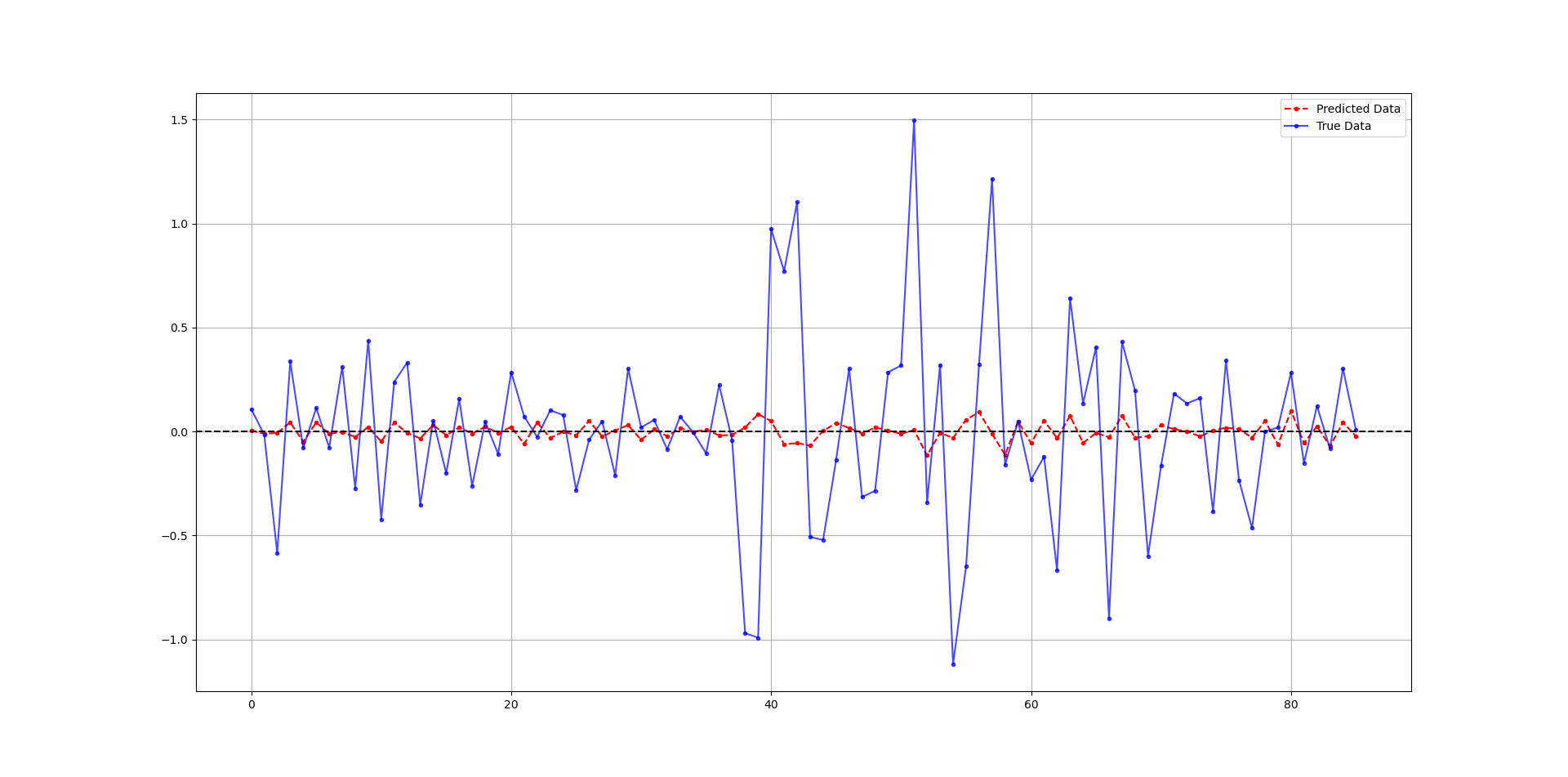

The following chart shows the predicted data (red) compared to real data. The hit ratio was about 60%.

Check out my newsletter that sends weekly directional views every weekend to highlight the important trading opportunities using a mix between sentiment analysis (COT report, put-call ratio, etc.) and rules-based technical analysis.

SGD regression is typically applied in linear regression problems but can also be used for other forms of regression models, such as logistic regression. It is particularly useful when working with very large datasets where traditional methods may be too slow or computationally expensive.