Gradient Boosting Regression in Python

Presenting and Coding a Machine Learning Model on Time Series

This article will discuss a machine learning model referred to as Gradient Boosting Regression (as opposed to Histogram-based GBR from last week). We will download a time series from an online source, transform it (i.e. make it stationary) and will simply apply the model’s tools to forecast t+1 values at each time step. We will just apply a simple performance evaluation tool, that is the accuracy (or hit ratio).

---

Intuition of the Model

Gradient Boosting Regressor is a powerful machine learning method used for predicting continuous values—like housing prices, stock trends, or energy consumption. At its core, it builds a strong model by combining many simple ones, usually decision trees. But instead of building all the trees at once, it builds them one after another, each time learning from the mistakes of the previous trees. That’s where the “boosting” comes in—it’s an iterative process that focuses on fixing the errors made so far.

Here’s how it works in plain terms: Imagine you're trying to predict someone’s weight based on their height, age, and exercise habits. The first tree might make a rough guess, but it won’t get everything right. The second tree then looks at where the first one got it wrong and tries to correct those specific errors. This keeps going, with each new tree zooming in on the remaining mistakes. Over time, the model gets better and better, like a team of editors polishing a rough draft into a clean final copy.

What makes Gradient Boosting especially effective is how it handles complex patterns and interactions between variables. It doesn’t assume a straight-line relationship between input and output, and it can dig deep into the data to find subtle trends. You can also tweak how much each tree contributes (called the learning rate), how complex each tree is (depth), and how many trees to build—giving you a lot of control over performance and overfitting.

In short, Gradient Boosting Regressor is like a smart, adaptive learner that builds up knowledge step by step to deliver sharp, accurate predictions.

Do you want to master Deep Learning techniques tailored for time series, trading, and market analysis🔥? My book breaks it all down from basic machine learning to complex multi-period LSTM forecasting while going through concepts such as fractional differentiation and forecasting thresholds. Get your copy here 📖!

Using the Model to Forecast Time Series

Let’s use the model in Python to apply the returns of a time series. We’ll choose the returns of S&P 500 for this task, while knowing that it’s almost impossible to accurately predict such a chaotic dataset with simple models, but we will do it just to make the models work. The plan of attack is as follows:

• Download the time series.

• Take the returns of the prices to make it stationary (an important condition of machine learning forecasting).

• Split the data into training and test sets.

• Fit and predict.

• Evaluate and plot the predictions.

Use the following code to conduct the experiment.

from sklearn.ensemble import GradientBoostingRegressor
import pandas_datareader as pdr
import numpy as np
import matplotlib.pyplot as plt

def data_preprocessing(data, num_lags, train_test_split):
    # Prepare the data for training
    x = []
    y = []
    for i in range(len(data) - num_lags):
        x.append(data[i:i + num_lags])
        y.append(data[i+ num_lags])
    # Convert the data to numpy arrays
    x = np.array(x)
    y = np.array(y)
    # Split the data into training and testing sets
    split_index = int(train_test_split * len(x))
    x_train = x[:split_index]
    y_train = y[:split_index]
    x_test = x[split_index:]
    y_test = y[split_index:]
    return x_train, y_train, x_test, y_test 

start_date = '1960-01-01'
end_date   = '2020-01-01'

# Import the data
data = (pdr.get_data_fred('SP500', start = start_date, end = end_date).dropna())
data = np.diff(data['SP500'])

# Train-test split
x_train, y_train, x_test, y_test = data_preprocessing(data, 100, 0.80)

# Create and train the model
model = GradientBoostingRegressor()
model.fit(x_train, y_train)

# Make predictions on the test set
y_pred = model.predict(x_test)

# Evaluate the model
same_sign_count = np.sum(np.sign(y_pred) == np.sign(y_test)) / len(y_test) * 100
print('Hit Ratio = ', same_sign_count, '%')

# Plot the actual vs. predicted values
plt.figure(figsize=(12, 6))
plt.plot(y_test[-50:], label = 'Actual', color = 'blue')
plt.plot(y_pred[-50:], label = 'Predicted', color = 'red')
plt.legend()
plt.title('Actual vs. Predicted')
plt.ylabel('Value')
plt.show()
plt.grid()
plt.axhline(y = 0, color = 'black')

The following is the plot that compares the real data from the test set and the predicted data.

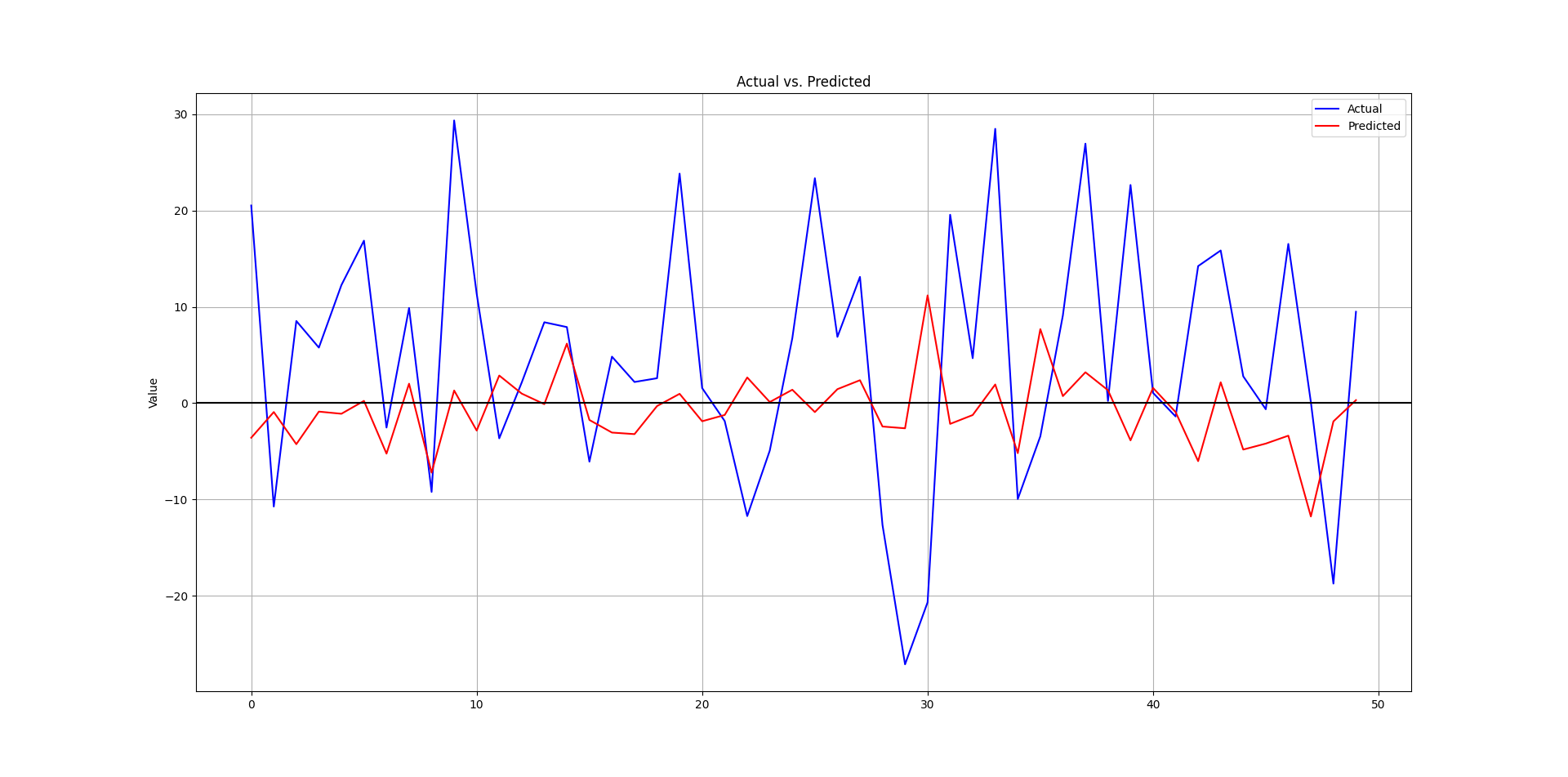
The following output shows the hit ratio.

44.87%

Every week, I analyze positioning, sentiment, and market structure. Curious what hedge funds, retail, and smart money are doing each week? Then join hundreds of readers here in the Weekly Market Sentiment Report 📜 and stay ahead of the game through chart forecasts, sentiment analysis, volatility diagnosis, and seasonality charts.

Free trial available🆓