Fundamental Analysis in Python - The ISM PMI Technique
Using the ISM PMI as a Predictor of the Currency Market
Fundamental analysis is a crucial part in investments and can also be a timing tool in some instances. The basic idea is that since it targets the very long-term, timing the market is either not important or left to technical analysis. However, tools such as the ISM PMI, when used right, may provide some tops and bottoms on some markets. In this article, we will discuss the ISM PMI and then try to see whether it provides good signals on the US Dollar or not.
The ISM PMI
The institute for supply management provides a monthly survey called the purchasing manager’s index abbreviated to PMI, which is based on questions asked to 400 representatives of industrial companies about the current and future trend of their different activities. It is composed of 5 components that can also be analyzed individually:
New orders — 30% weight.
Production — 25% weight.
Employment — 20% weight.
Supplier Deliveries — 15% weight.
Inventories — 10% weight.
Typically, we interpret the index as 50 being the neutral state of the economy (neither growing and neither shrinking). A reading above 50 indicates an expansion in manufacturing and a reading below 50 indicates shrinking in manufacturing. The PMI tends to peak before the whole economy with a lead of 6–12 months, which makes it an astonishing leading indicator (more than 0.70 correlation with the US GDP). It is also correlated with the S&P500 and negatively correlated with the US Dollar which is represented by the DXY.
One way to use the PMI in FX trading is by using the following intuition: If the values are growing, then it is most likely that the economy is improving, which in turn would imply that we should start to be concerned with inflationary problems. The PMI is ordinarily used as a contrarian indicator with the US Dollar even though in the short-term, a positive PMI value tends to be associated with a rise in the dollar.
For example, if the reading of the indicator is around 60 then we should expect a peak to happen anytime soon, as well as a bottom in the Dollar index if it has been trending down (an expected weakening of the economy is associated with deflation and the rise of the currency all else equal). In the next part, we will see how to download the full historical data of the ISM PMI as well as the US Dollar index, also known as the DXY.
For the complete collection of candlestick patterns in detail with back-tests and technical strategies, you can check out my newest book with O’Reilly Media. The book features a huge number of classic and modern candlestick patterns as it dwelves into the realm of technical analysis with different trading strategies. The book comes with its own GitHub and is dynamic in nature as it is continuously updated and questions are answered on the O’Reilly platform promptly.
Mastering Financial Pattern Recognition
Amazon.com: Mastering Financial Pattern Recognition eBook : Kaabar, Sofien: Kindle Storewww.amazon.com
Downloading DXY and ISM PMI Historical Data
The free way to download the historical data on the ISM PMI is through Quandl. They have it on the freely downloadable list of indicators. The way I do it is by choosing csv and then cleaning it a bit and transforming it into an xlsx (Excel) file. We can now download historical monthly data on the DXY from the current link at Investing website. We just need to select the date period and then click on download or simply copy the whole columns and then paste them in excel before cleaning up as well.
The DXY is the US Dollar index, a weighted basked that tracks the dollar’s strength.
The final step is putting the ISM PMI and DXY columns together so that we import them into the Python interpreter (in my case, it is SPYDER 4.0). Make sure to have this format:
We need to remove all the descriptions and keep OHLC data of the Dollar first and then at the end simply keep the monthly ISM PMI readings.
Visualizing & Analyzing in Python
The next step is to open the Python interpreter and import the excel file which we can call Data. Make sure that the directory is set to where the excel file is stored before running the below code:
import numpy as np
import pandas as pd
# Importing the excel file as a Data frame
Data = pd.read_excel('Data.xlsx')# Converting to a numpy array
Data = np.array(Data)Let us plot them together in the same chart.
We can notice the negative correlation visually. The latest 13-period correlation coefficient is -0.88 suggesting a strong negative correlation on the monthly horizon.
“A deflationary economy can be favorable for the appreciation of the USD while and inflationary (expanding) economical environment may stimulate a weakening of the Dollar.”
Now, we will look at two ways of analysis, the first that I call a fixed barrier analysis and the second, the variable barrier analysis.
Strategy #1: Fixed Barrier Analysis ISM PMI
The historical barriers on the ISM PMI were around 62–60 as the upper barrier and 42–40 as the lower barrier. These can be considered as the economic growth subjective boundaries as we generally see a reversal of trend around them. The low of the 2008 crisis was seen around 40–35 readings on the ISM PMI. Therefore, following our logic with the US Dollar, we will have the following conditions:
A bullish signal is triggered whenever the PMI reaches the area of 62–60.
A bearish signal is triggered whenever the PMI reaches the area of 42–40.
upper_barrier    = 60
lower_barrier    = 42
def signal(Data, what, buy, sell):
for i in range(len(Data)):
if Data[i, what] < lower_barrier and Data[i - 1, what] > lower_barrier and Data[i - 2, what] > lower_barrier :
Data[i, sell] = -1
if Data[i, what] > upper_barrier and Data[i - 1, what] < upper_barrier and Data[i - 2, what] < upper_barrier :
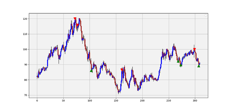
Data[i, buy] = 1The rare signals do seem to correlate with tops and bottoms with the recent USD bearish move these last months predicted by the ISM PMI.
Strategy #2: Variable Barrier Analysis ISM PMI
John Bollinger has created his famous bands that are used in technical analysis, although they come mainly from the field of descriptive statistics. We can use the Bollinger bands to get objective signals as well. This way, we can simply say that the ISM PMI has reached its 2-standard deviation barrier and might reverse. However, I have found that the best setup occurs with a lookback period of 150. The below signal chart shows the results:
A bullish signal is triggered whenever the PMI reaches the upper 150-period Bollinger Band.
A bearish signal is triggered whenever the PMI reaches the lower 150-period Bollinger Band.
boll_lookback = 150
standard_distance = 2
def signal(Data, what, upper_boll, lower_boll, buy, sell):
for i in range(len(Data)):
if Data[i, what] > Data[i, upper_boll] and Data[i - 1, what] < Data[i - 1, upper_boll] and Data[i - 2, what] < Data[i - 2, upper_boll]:
Data[i, buy] = 1
if Data[i, what] < Data[i, lower_boll] and Data[i - 1, what] > Data[i - 1, lower_boll] and Data[i - 2, what] > Data[i - 2, lower_boll]:
Data[i, sell] = -1
Let us quickly discuss the Bollinger bands and the code needed to create them. When prices move, we can calculate a moving average (mean) around them so that we better understand their position regarding their mean.
By doing this we can also calculate where do they stand statistically. But first we need to understand the concept of the normal distribution curve which is the essence of statistics and the foundation of statistical theory.
The above curve shows the number of values within a number of standard deviations. For example, the area shaded in red represents around 1.33x of standard deviations away from the mean of zero. We know that if data is normally distributed then:
About 68% of the data falls within 1 standard deviation of the mean.
About 95% of the data falls within 2 standard deviations of the mean.
About 99% of the data falls within 3 standard deviations of the mean.
Presumably, this can be used to approximate the way to use financial returns data, but studies show that financial data is not normally distributed but at the moment we can assume it is so that we can use such indicators. The issue with the method does not hinder much its usefulness.
Hence, the Bollinger bands are simple a combination of a moving average that follows prices and a moving standard deviation(s) band that moves alongside the price and the moving average. To calculate the two Bands, we use the following relatively simple formulas:
With the constant being the number of standard deviations that we choose to envelop prices with. By default, the indicator calculates a 20-period simple moving average and two standard deviations away from the price, then plots them together to get a better understanding of any statistical extremes. This means that on any time, we can calculate the mean and standard deviations of the last 20 observations we have and then multiply the standard deviation by the constant. Finally, we can add and subtract it from the mean to find the upper and lower band.
def ma(Data, lookback, what, where):

    for i in range(len(Data)):
      try:
        Data[i, where] = (Data[i - lookback + 1:i + 1, what].mean())

            except IndexError:
                pass
    return Data
def volatility(Data, lookback, what, where):
for i in range(len(Data)):
try:
Data[i, where] = (Data[i - lookback + 1:i + 1, what].std())
except IndexError:
pass
return Datadef BollingerBands(Data, boll_lookback, standard_distance, what, where):
# Calculating mean
ma(Data, boll_lookback, what, where)
# Calculating volatility
volatility(Data, boll_lookback, what, where + 1)
Data[:, where + 2] = Data[:, where] + (standard_distance * Data[:, where + 1])
Data[:, where + 3] = Data[:, where] - (standard_distance * Data[:, where + 1])
return Data


