

Many time series contain repeated structure: daily demand cycles, weekly traffic patterns, seasonal temperature patterns, production rhythms, or market microstructure effects. Fourier methods are designed to represent a signal as a sum of oscillations. This makes them a natural tool for detecting and forecasting cyclical behavior.
This article introduces a causal Fourier forecasting method. The word causal means that the forecast made at time ttt only uses observations available up to time ttt. We will generate a synthetic time series with hidden cycles, estimate its dominant frequencies using a trailing window, and use those frequencies to forecast future values.
The method is intentionally simple. It is not meant to beat specialized forecasting models in every setting. Its value is interpretability: it shows how much of a time series can be explained by cycles.
The problem: forecasting repeated structure
Suppose we observe a time series:
and want to forecast future values
A common assumption is that the future resembles the past in some structured way. Fourier methods focus on one particular kind of structure: periodicity.
For example, a signal might contain:
a slow trend,
a weekly cycle,
a shorter intraday cycle,
random noise.
In plain language, Fourier analysis asks:
Can this time series be approximated as a combination of waves?
If the answer is yes, then we can estimate those waves from recent historical data and extend them forward.
Intuition: decomposing a signal into waves
A sine wave is one of the simplest repeating patterns:
where:
A is the amplitude, or the strength of the oscillation,
f is the frequency, or how fast the wave repeats,
t is time,
ϕ is the phase, or where the wave is in its cycle.
A Fourier model approximates a signal as a sum of many such waves:
This is useful because complicated repeated behavior can often be built from simpler periodic components.
The key idea for forecasting is straightforward:
Look at the recent past.
Estimate the dominant cycles.
Continue those cycles into the future.
I built Quant Atlas to cut through market noise.
No opinions. Just quantitative, robust, quality forecasts.
Try it yourself in real time.
The Discrete Fourier Transform
For a finite window of N observations
where yn is a recent segment of the original time series, the Discrete Fourier Transform, or DFT, is defined as:
The inverse transform reconstructs the signal:
Each coefficient Xk tells us how much of frequency k/N is present in the signal.
The magnitude
measures the strength of that frequency. The phase
tells us where that oscillation is located in its cycle.
Making the Fourier method causal
A standard Fourier transform is usually applied to a full series. That is not causal if we are pretending to forecast through time, because it would allow information from the future to influence the past.
To avoid this, we use a trailing window. At time ttt, we only use:
Then we compute the DFT on this window and forecast forward.
Formally, define the window available at time t as:
We compute:
Then we keep only the strongest frequencies and extrapolate them into the future.
A simple forecast at horizon h is:
where K is the set of selected dominant frequencies.
This expression uses the index N−1+h because the most recent observation in the window corresponds to local time N−1, so the next value corresponds to N.
Synthetic time series with detectable cycles
We will generate a time series with two known cycles:
A slow cycle with period 50.
A faster cycle with period 12.
The signal is:
where ϵ is random noise:
The linear term 0.03t adds a mild trend. The two sine terms create repeating structure. The noise term makes the problem realistic.
Python implementation
The script below:
Generates synthetic data.
Builds a causal Fourier forecaster.
Forecasts one step ahead using a trailing window.
Plots the original series, forecasts, and detected frequency strengths.
import numpy as np
import pandas as pd
import matplotlib.pyplot as plt

np.random.seed(7)

n = 500
t = np.arange(n)

trend = 0.03 * t
cycle_slow = 2.0 * np.sin(2 * np.pi * t / 50)
cycle_fast = 0.8 * np.sin(2 * np.pi * t / 12)
noise = np.random.normal(0, 0.6, size=n)

x = trend + cycle_slow + cycle_fast + noise

data = pd.DataFrame({
    "t": t,
    "x": x
})

def fourier_forecast_one_step(window, n_freqs=5, detrend=True):
    """
    Forecast the next value using a causal trailing-window Fourier model.

    Parameters
    ----------
    window : array-like
        Most recent observations available up to current time.
    n_freqs : int
        Number of dominant positive frequencies to keep.
    detrend : bool
        If True, remove a linear trend before applying the FFT,
        then extrapolate the trend one step forward.

    Returns
    -------
    forecast : float
        One-step-ahead forecast.
    freqs : ndarray
        Positive Fourier frequencies.
    amplitudes : ndarray
        Amplitudes associated with the positive frequencies.
    """
    y = np.asarray(window, dtype=float)
    N = len(y)
    idx = np.arange(N)

    if detrend:
        # Fit y = a * idx + b using only the current window.
        a, b = np.polyfit(idx, y, deg=1)
        trend_fit = a * idx + b
        y_centered = y - trend_fit
        next_trend = a * N + b
    else:
        y_centered = y - np.mean(y)
        next_trend = np.mean(y)

    # FFT of the detrended signal.
    coeffs = np.fft.rfft(y_centered)
    freqs = np.fft.rfftfreq(N, d=1.0)

    # Convert complex coefficients to amplitudes.
    amplitudes = np.abs(coeffs) / N

    # Exclude the zero-frequency term.
    positive = np.arange(1, len(freqs))

    # Select dominant frequencies by amplitude.
    selected = positive[np.argsort(amplitudes[positive])[-n_freqs:]]

    # Forecast local time N, which is one step after the window.
    future_idx = N
    reconstructed = 0.0

    for k in selected:
        amp = 2 * np.abs(coeffs[k]) / N
        phase = np.angle(coeffs[k])
        reconstructed += amp * np.cos(2 * np.pi * freqs[k] * future_idx + phase)

    forecast = next_trend + reconstructed

    return forecast, freqs, amplitudes

window_size = 128
n_freqs = 5

forecasts = np.full(n, np.nan)

for current_time in range(window_size, n - 1):
    window = x[current_time - window_size + 1 : current_time + 1]
    forecasts[current_time + 1], _, _ = fourier_forecast_one_step(
        window,
        n_freqs=n_freqs,
        detrend=True
    )

data["fourier_forecast"] = forecasts

plt.figure(figsize=(12, 5))
plt.plot(data["t"], data["x"], label="Actual", linewidth=1.5)
plt.plot(data["t"], data["fourier_forecast"], label="Causal Fourier forecast", linewidth=2)
plt.axvline(window_size, linestyle="--", linewidth=1, label="Forecasting starts")
plt.title("Causal Fourier one-step-ahead forecast")
plt.xlabel("Time")
plt.ylabel("Value")
plt.legend()
plt.tight_layout()
plt.show()

last_window = x[-window_size:]
_, freqs, amplitudes = fourier_forecast_one_step(
    last_window,
    n_freqs=n_freqs,
    detrend=True
)

positive = freqs > 0
periods = 1 / freqs[positive]

plt.figure(figsize=(12, 5))
plt.stem(periods, amplitudes[positive])
plt.xlim(0, 80)
plt.title("Frequency strength expressed as period length")
plt.xlabel("Period")
plt.ylabel("Amplitude")
plt.tight_layout()
plt.show()

eval_data = data.dropna().copy()
mae = np.mean(np.abs(eval_data["x"] - eval_data["fourier_forecast"]))
rmse = np.sqrt(np.mean((eval_data["x"] - eval_data["fourier_forecast"]) ** 2))

print(f"MAE:  {mae:.3f}")
print(f"RMSE: {rmse:.3f}")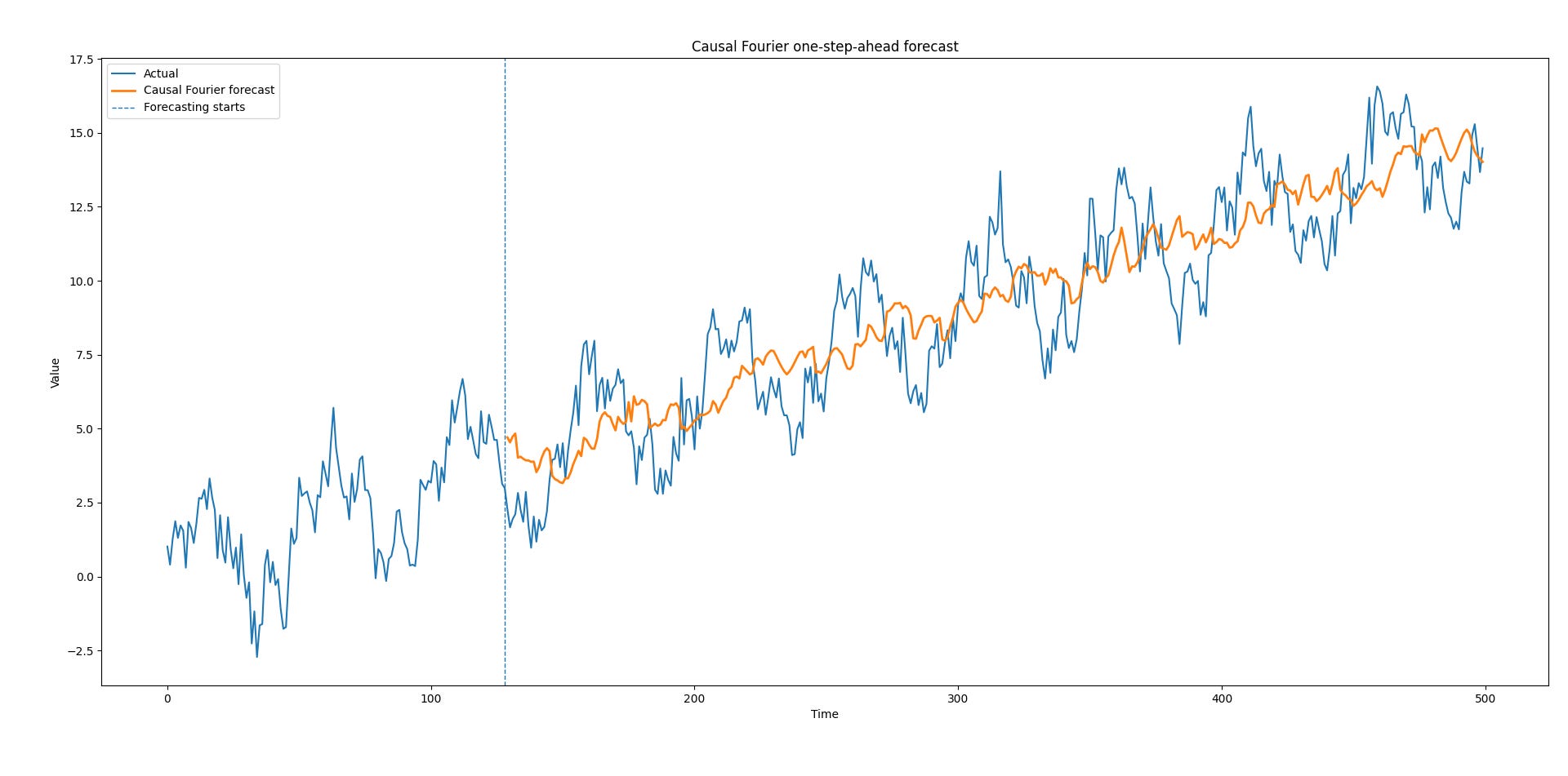
The first chart compares the actual signal with the one-step-ahead Fourier forecast. The forecast should track the cyclical movement reasonably well because the synthetic data was designed to contain stable periodic components.
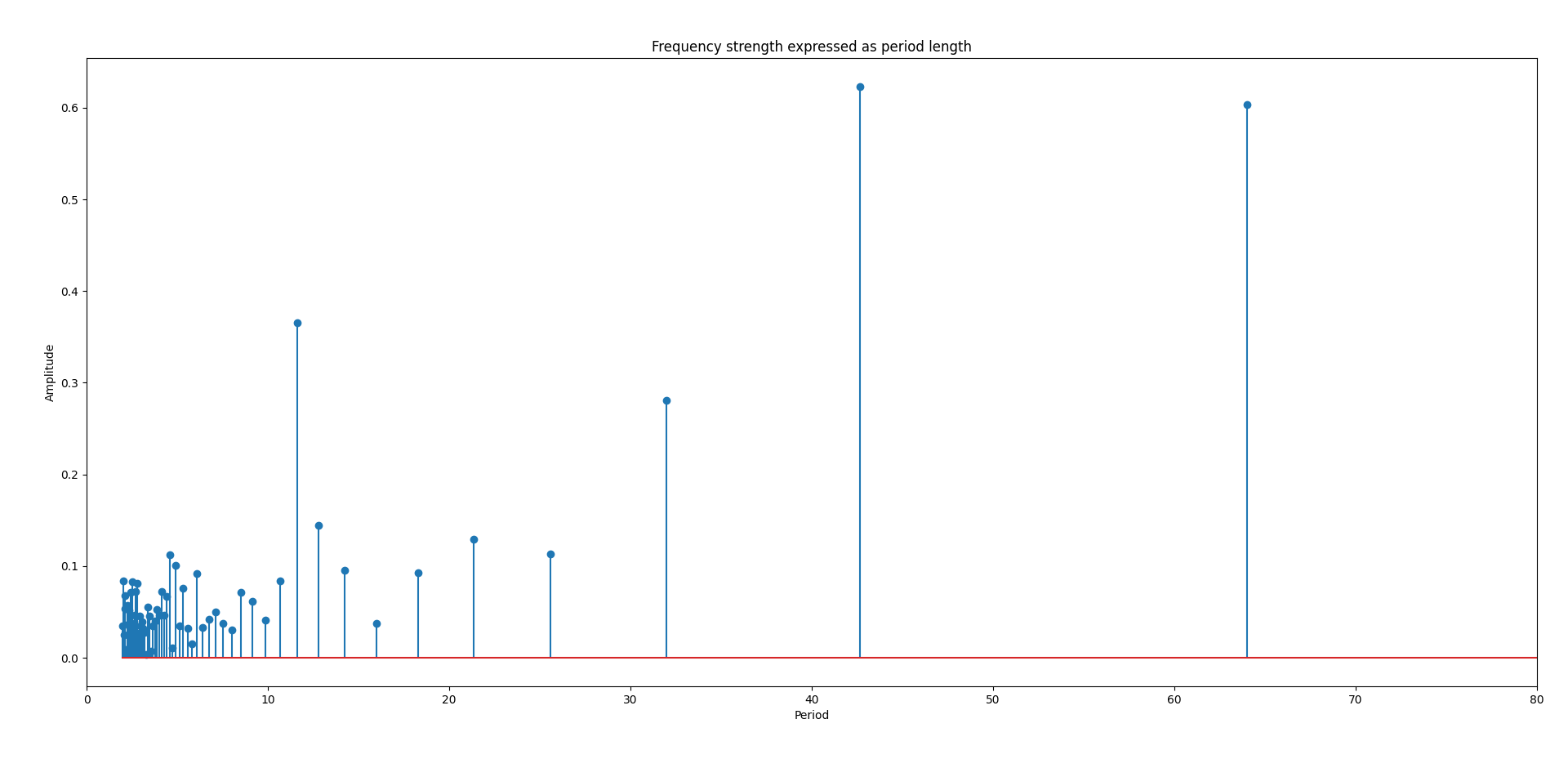
The second chart expresses Fourier frequencies as periods. Since the true signal contains periods near 50 and 12, the amplitude plot should show noticeable peaks near those values.
The peaks will not be perfect. Noise, finite window length, trend, and frequency resolution all affect the result.
The frequency resolution of the DFT is:
That means longer windows can distinguish nearby frequencies more precisely. But longer windows also adapt more slowly when the underlying cycles change.
This is one of the central tradeoffs in time-series signal processing.
Why detrending matters
Fourier methods assume that the signal can be represented by oscillations around a stable level. A strong trend can dominate the transform and distort the frequency estimates.
That is why the code removes a local linear trend before computing the FFT.
Inside each window, we fit:
Then we apply the FFT to the residual:
The forecast is then:
In plain terms: we separately estimate the direction of movement and the repeating pattern around that movement.
Strengths of causal Fourier forecasting
Interpretability
Fourier methods tell us which cycles are present. This is different from many black-box forecasting methods, which may produce accurate predictions without explaining the underlying structure.
With Fourier analysis, we can say:
That makes the method useful not only for prediction, but also for diagnosis.
Efficient computation
The Fast Fourier Transform computes the DFT efficiently. For a window of size N, the FFT has complexity:
This is efficient enough for many practical rolling-window applications.
For real-time systems, one can go further and use the Sliding DFT, which updates Fourier coefficients recursively as new samples arrive.
Good fit for stable seasonality
Fourier methods work well when cycles are stable or slowly changing. They are often useful in demand forecasting, traffic analysis, electricity consumption, temperature modeling, and sensor monitoring.
Limitations
Weak performance when cycles are unstable
If the dominant period changes quickly, a Fourier model estimated from a fixed window may lag behind the true process.
For example, a cycle with period 50 that gradually shifts to period 35 may be poorly represented unless the window is short enough to adapt.
Sensitivity to window size
The window size N controls the balance between frequency precision and adaptability.
A long window gives better frequency resolution:
But it also uses older data, which may no longer be relevant.
A short window adapts faster, but it has poorer frequency resolution and noisier estimates.
Boundary effects
When forecasting from a finite window, the model implicitly assumes that the observed segment is representative of the cycle. If the window starts or ends at an unusual point, the forecast can be distorted.
Windowing functions can help reduce spectral leakage, but they introduce their own tradeoffs.
Not designed for shocks
Fourier models are smooth and periodic. They are not naturally suited for sudden jumps, regime changes, or one-off shocks.
This is where wavelet methods are often more appropriate.
Financial market applications
Financial markets are a difficult setting for Fourier forecasting because price series are noisy, adaptive, and often close to random at short horizons. Still, Fourier methods can be useful if applied carefully.
The key is not to think of Fourier analysis as a magic price predictor. It is better understood as a tool for detecting cyclicality, seasonality, and market rhythms.
Intraday seasonality
Market activity often follows intraday patterns. Volume, volatility, and spreads can behave differently near the open, midday, and close.
Fourier features can model these repeating intraday effects. For example, instead of forecasting raw returns, one might forecast:
or
These quantities often have stronger seasonal structure than prices themselves.
Volatility cycles
Volatility can cluster and sometimes exhibit periodic behavior around scheduled events, trading sessions, or macroeconomic announcement cycles.
A causal Fourier model could be applied to a rolling estimate of volatility:
where rt is the return at time t.
The goal would not be to forecast the exact next return, but to estimate whether risk is likely to rise or fall based on recent cyclical structure.
Feature engineering for trading models
Fourier components can be used as features in a broader model. For example:
These features can then be passed into a regression, classification, or risk model.
This is often more realistic than using the Fourier forecast directly as a trading signal.
Avoiding look-ahead bias
The causal structure is essential in finance. Any transform that uses future data will produce misleading backtests.
Common sources of look-ahead bias include:
computing Fourier coefficients on the full series,
using centered windows,
normalizing with full-sample statistics,
selecting frequencies using the entire dataset,
smoothing predictions with future observations.
A valid financial backtest must ensure that every feature at time ttt uses only data available at or before time t.