Market forecasting in technical analysis can be done in many ways. Among these techniques are divergences. However, divergences are known contrarian techniques but they can also be tweaked into becoming trend following techniques. This article shows the intuition and the code of this tweak.
I have released a new book after the success of my previous one “Trend Following Strategies in Python”. It features advanced contrarian indicators and strategies with a GitHub page dedicated to the continuously updated code. If you feel that this interests you, feel free to visit the below Amazon link (which contains a sample), or if you prefer to buy the PDF version, you could check the link at the end of the article.
Contrarian Trading Strategies in Python
Amazon.com: Contrarian Trading Strategies in Python: 9798434008075: Kaabar, Sofien: Bookswww.amazon.com
The Stochastic Oscillator
The stochastic oscillator is a famous contrarian indicator based on 3 pieces of data: the close, the high, and the low. It is based on a normalization function where the output is a value bound between 0 and 100.
The concept revolves around subtracting the minimum value in a certain lookback period from the current value and dividing by the maximum value in the same lookback period minus the minimum value (the same in the nominator).
The stochastic oscillator takes this into another level and uses more information. The formula is as follows:
The next Figure shows the EURUSD values with the 14-period stochastic oscillator.
Generally, the Stochastic Oscillator is not charted in its raw form but with a double smoothing effect. Here’s how:
Calculate the raw stochastic oscillator using a lookback period of your choice (generally it is 5 or 14). We call this calculation, the %K.
Calculate a 3-period moving average on the raw stochastic oscillator.
Calculate a 3-period moving average on the %K values. We call this calculation, the %D.
The last two steps are what’s visible in charting platforms.
To code the oscillator, you need an OHLC numpy array composed of 4 columns and the below syntax:
def add_column(data, times):

    for i in range(1, times + 1):

        new = np.zeros((len(data), 1), dtype = float)

        data = np.append(data, new, axis = 1)
return datadef delete_column(data, index, times):
for i in range(1, times + 1):
data = np.delete(data, index, axis = 1) return datadef delete_row(data, number):
data = data[number:, ]
return datadef ma(data, lookback, close, position):
data = add_column(data, 1)
for i in range(len(data)):
try:
data[i, position] = (data[i - lookback + 1:i + 1, close].mean())
except IndexError:
pass
data = delete_row(data, lookback)
return datadef stochastic_oscillator(data,
lookback,
high,
low,
close,
position,
slowing = False,
smoothing = False,
slowing_period = 1,
smoothing_period = 1):
data = add_column(data, 1)
for i in range(len(data)):
try:
data[i, position] = (data[i, close] - min(data[i - lookback + 1:i + 1, low])) / (max(data[i - lookback + 1:i + 1, high]) - min(data[i - lookback + 1:i + 1, low]))
except ValueError:
pass
data[:, position] = data[:, position] * 100
if slowing == True and smoothing == False:
data = ma(data, slowing_period, position, position + 1)
if smoothing == True and slowing == False:
data = ma(data, smoothing_period, position, position + 1)
if smoothing == True and slowing == True:
data = ma(data, slowing_period, position, position + 1)
data = ma(data, smoothing_period, position + 1, position + 2)
data = delete_row(data, lookback) return dataTo simplify things, we can say that normalization only uses the closing price where values of 100 signify a highest close since a specified lookback period and values of 0 signify a lowest close since a specified lookback period. Similarly, the stochastic oscillator’s function incorporates the highs and the lows in its function so that a better version is given.
Make sure to focus on the concepts and not the code. You can find the codes of most of my strategies in my books. The most important thing is to comprehend the techniques and strategies.
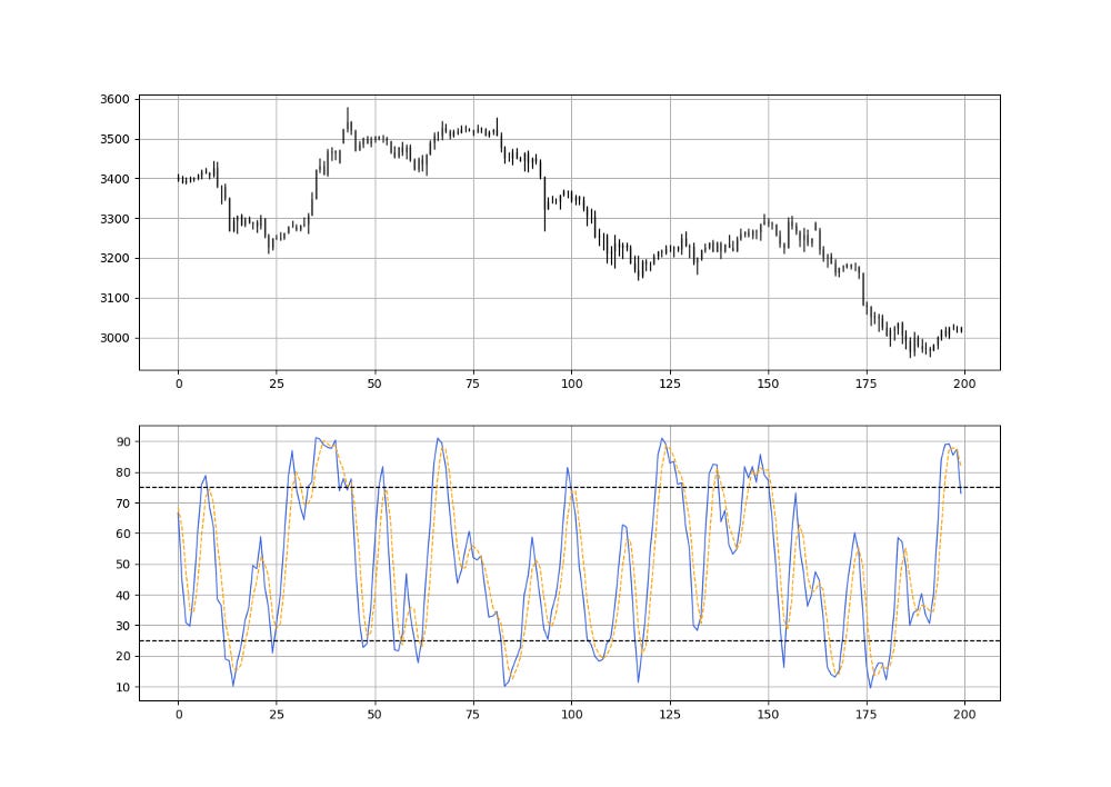
Let’s take a look at a 5-period stochastic oscillator (with its double smoothing from the two moving averages).
Hidden Divergences
The word divergence refers to a two or more elements that deviate from their past relationship. When two variables move at the same direction and they suddenly start moving in opposite directions, we tend to say that they have diverged.
The two variables we are referring to are the market price and the indicator that is based on it. Therefore, a divergence occurs whenever the past (usual) relationship between the market price and the indicator does not hold anymore.
Since the stochastic oscillator measures the momentum of the price, a divergence occurs whenever the market price falls and the stochastic oscillator rises or whenever the market price rises and the stochastic oscillator falls.
In essence, a divergence occurs because the acceleration (to the upside or downside) of a market is reduced and this can be seen in the indicator but not as clearly on the price action.
Therefore, for a normal divergence, the following trading conditions are typically used:
A long (buy) signal is generated whenever the market shapes two bottoms with the second bottom lower than the first one. In parallel, the indicator shapes two bottoms with the second bottom higher than the first one. This is referred to as a bullish divergence.
A short (sell) signal is generated whenever the market shapes two tops with the second top higher than the first one. In parallel, the indicator shapes two tops with the second top lower than the first one. This is referred to as a bearish divergence.
This means that a normal divergence is contrarian in nature. Let’s take a look at the conditions of a hidden divergence, a trend following technique:
A long (buy) signal is generated whenever the market shapes two bottoms with the second bottom higher than the first one (implying a bullish trend in-progress). In parallel, the indicator shapes two bottoms with the second bottom lower than the first one. This is referred to as a bullish hidden divergence.
A short (sell) signal is generated whenever the market shapes two tops with the second top lower than the first one (implying a bearish trend in-progress). In parallel, the indicator shapes two tops with the second top higher than the first one. This is referred to as a bearish hidden divergence.
Hence, a hidden divergence is an indicator of a better entry price within the on-going trend due to a short-term impulsive correction which causes the indicator to approach the extreme.
The next Figure shows signals from hidden divergences on BTCUSD.
The signal function used to create these signals are as follows:
def hidden_divergence(data, lower_barrier, upper_barrier, width):

    data = add_column(data, 10)

    for i in range(len(data)):

        try:
            if data[i, 5] < lower_barrier and data[i - 1, 5] > lower_barrier:

                for a in range(i + 1, i + width):

                    if data[a, 5] > lower_barrier:

                        for r in range(a + 1, a + width):

                            if data[r, 5] < lower_barrier and \
                            data[r, 5] < data[i, 5] and data[r, 3] > data[i, 3]:

                                for s in range(r + 1, r + width):

                                    if data[s, 5] > lower_barrier:
                                        data[s + 1, 6] = 1
                                        break

                                    else:
                                        break
                            else:
                                break
                        else:
                            break
                    else:
                        break

        except IndexError:
            pass

    for i in range(len(data)):

        try:
            if data[i, 5] > upper_barrier  and data[i - 1, 5] < upper_barrier:

                for a in range(i + 1, i + width):

                    if data[a, 5] < upper_barrier:
                        for r in range(a + 1, a + width):
                            if data[r, 5] > upper_barrier and \
                            data[r, 5] > data[i, 5] and data[r, 3] < data[i, 3]:
                                for s in range(r + 1, r + width):

                                    if data[s, 5] < upper_barrier:
                                        data[s + 1, 7] = -1
                                        break
                                    else:
                                        break
                            else:
                                break
                        else:
                            break
                    else:
                        break
        except IndexError:
            pass

    return data
The next Figure shows the signals generated on USDCAD. Notice how the hidden divergence tends to follow the trend.
Summary
To summarize up, what I am trying to do is to simply contribute to the world of objective technical analysis which is promoting more transparent techniques and strategies that need to be back-tested before being implemented. This way, technical analysis will get rid of the bad reputation of being a subjective and scientifically unfounded.
I recommend you always follow the the below steps whenever you come across a trading technique or strategy:
Have a critical mindset and get rid of any emotions.
Back-test it using real life simulation and conditions.
If you find potential, try optimizing it and running a forward test.
Always include transaction costs and any slippage simulation in your tests.
Always include risk management and position sizing in your tests.
Finally, even after making sure of the above, stay careful and monitor the strategy because market dynamics may shift and make the strategy unprofitable.
For the PDF alternative, the price of the book is 9.99 EUR. Please include your email in the note before paying so that you receive it on the right address. Also, once you receive it, make sure to download it through google drive.
Pay Kaabar using PayPal.Me
If you accept cookies, we’ll use them to improve and customize your experience and enable our partners to show you…www.paypal.com


