Financial Signal Processing in Python VI - Applying the Wiener Filter on Time Series

Part V of Decomposing Time Series and Understanding their Components

This article will be the part VI of a series of articles that present the signal processing field in an easy and straightforward manner. Financial Signal Processing (FSP) is the application of signal processing techniques to financial time series—like stock prices, returns, volatility, or economic indicators.

It treats price movements like signals—similar to audio—and applies filters, transformations, and models to extract hidden patterns, reduce noise, or make forecasts.

There are many concepts in FSP that are worth discussing, and throughout these special articles, I will try to present each one with functioning code that shows how to use and interpret it:

• Decomposition

  • Empirical Mode Decomposition (EMD)

  • Principal Component Analysis (PCA)

• Filters

  • Moving Averages

  • Kalman Filter

  • Wiener Filter 👈🏻

• Spectral Analysis

  • Fourier Transform

  • Wavelet Transform

• Denoising

  • Wavelet Denoising

  • Savitzky–Golay Filter

• Anomaly Detection

  • Recurrence Plots

  • Entropy

  • Signal Spikes

---

Introduction to the Wiener Filter

The Wiener Filter is a fundamental tool in signal processing and time series forecasting. It was introduced by Norbert Wiener in the 1940s and is essentially the optimal linear filter for estimating or predicting a desired signal from a noisy observation. Its goal is to minimize the mean squared error (MSE) between the predicted signal and the true signal.

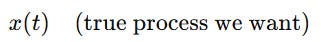
Suppose we have a signal (or what we refer to as values within time steps):

But we only observe:

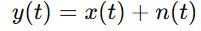
where n(t) is noise. We want to find a linear filter h such that:

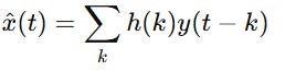
minimizes:

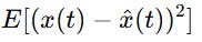
The first principle of the Wiener filter is that it gives the best possible linear estimate under MSE. The second principle is that it uses only autocorrelation and cross-correlation (second-order statistics), not full distributions. The third one is that it works best when signals/noise are stationary.

In time series, the Wiener filter essentially reduces to the linear least squares predictor. For stationary processes:

• If you want to filter noise, you use it as a denoiser.

• If you want to predict future values, you design the Wiener filter as a forward predictor (related to AR models and Kalman filtering).

Before we move on to creating the algorithm, let’s quickly understand the MSE. The MSE is a common way to measure how well a model’s predictions match the actual data.

• yi = true value

• y^i​ = predicted value

• n = number of samples

Squaring ensures all errors are positive (so under-predicting and over-predicting don’t cancel out).

Do you want to master Deep Learning techniques tailored for time series, trading, and market analysis🔥? My book breaks it all down from basic machine learning to complex multi-period LSTM forecasting while going through concepts such as fractional differentiation and forecasting thresholds. Get your copy here 📖!

---

Application of the Machine Learning Model

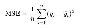
We will generate a random walk then apply the Wiener filter to smooth it out. Finally, we will run an XGBoost regression on the latter and use a multi-period forecasting technique to project a future trajectory (instead of a t+1 forecats). For this, we will sumply use the prediction as a feature so that we continue doing it into the future.

We previously defined and introduced XGBoost, therefore we will omit it from this post.

⚠️ Note: Random walks are non-stationary and not ideal for Wiener filtering. In practice, Wiener filtering works best for stationary signals (e.g., AR processes). But this gives a clear demo.

Use the following code to implement the experiment, knowing that this is just a basic implementation (as many other more complex techniques such as multi-layered forecasting can be applied).

import numpy as np
import matplotlib.pyplot as plt
from scipy.signal import wiener
from xgboost import XGBRegressor

# 1. Simulate random walk with noise
np.random.seed(123)
n = 300
steps = np.random.normal(0, 1, size=n)
random_walk = np.cumsum(steps)
noise = np.random.normal(0, 2, size=n)
observed = random_walk + noise

# 2. Apply Wiener filter
filtered = wiener(observed, mysize=7)

# 3. Prepare lagged dataset for XGBoost
def create_lagged_features(series, window=10):
    X, y = [], []
    for i in range(len(series) - window):
        X.append(series[i:i+window])
        y.append(series[i+window])
    return np.array(X), np.array(y)

window = 100
X, y = create_lagged_features(filtered, window)

# Split into train and test
split = int(0.8 * len(X))
X_train, X_test = X[:split], X[split:]
y_train, y_test = y[:split], y[split:]

# 4. Train XGBoost model
model = XGBRegressor(
    n_estimators=300,
    learning_rate=0.05,
    max_depth=4,
    subsample=0.8,
    colsample_bytree=0.8,
    random_state=42
)
model.fit(X_train, y_train)

# 5. Predict test values
y_pred_test = model.predict(X_test)

# 6. Recursive multi-step future prediction
m = 20  # predict next 20 steps
last_window = list(filtered[-window:])
pred_future = []
for _ in range(m):
    next_val = model.predict(np.array(last_window[-window:]).reshape(1, -1))[0]
    pred_future.append(next_val)
    last_window.append(next_val)

# 7. Plot results
plt.figure(figsize=(12,6))
plt.plot(random_walk, label="True Random Walk", linewidth=2)
plt.plot(filtered, label="Wiener Filtered", linewidth=2)
plt.plot(range(split+window, split+window+len(y_pred_test)), y_pred_test, label="XGBoost Test Prediction")
plt.plot(np.arange(n, n+m), pred_future, 'r--', label="XGBoost Future Forecast")
plt.legend()
plt.title("Wiener Filter + XGBoost Forecast on Random Walk")
plt.show()
plt.grid()

The following chart shows the output.

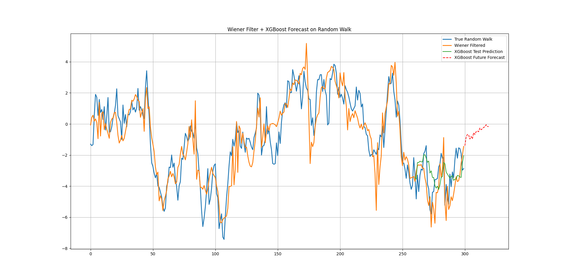
Each value is predicted one step at a time, using the previous prediction as input for the next.

Every week, I analyze positioning, sentiment, and market structure. Curious what hedge funds, retail, and smart money are doing each week? Then join hundreds of readers here in the Weekly Market Sentiment Report 📜 and stay ahead of the game through chart forecasts, sentiment analysis, volatility diagnosis, and seasonality charts.

Free trial available🆓