Financial Signal Processing in Python III - Principal Component Analysis

Part III of Decomposing Time Series and Understanding their Components

This article will be the part III of a series of articles that present the signal processing field in an easy and straightforward manner. Financial Signal Processing (FSP) is the application of signal processing techniques to financial time series—like stock prices, returns, volatility, or economic indicators.

It treats price movements like signals—similar to audio—and applies filters, transformations, and models to extract hidden patterns, reduce noise, or make forecasts.

There are many concepts in FSP that are worth discussing, and throughout these special articles, I will try to present each one with functioning code that shows how to use and interpret it:

• Decomposition

  • Empirical Mode Decomposition (EMD)

  • Principal Component Analysis (PCA) 👈🏻

• Filters

  • Moving Averages

  • Kalman Filter

  • Wiener Filter

• Spectral Analysis

  • Fourier Transform

  • Wavelet Transform

• Denoising

  • Wavelet Denoising

  • Savitzky–Golay Filter

• Anomaly Detection

  • Recurrence Plots

  • Entropy

  • Signal Spikes

---

The Theory of Principal Component Analysis

Principal Component Analysis (PCA) is a way to take messy, high-dimensional data and turn it into something simpler — without losing too much important information.
Think of it like compressing a giant messy spreadsheet into a few summary columns that still explain most of the patterns in the data.

If you have data with many variables x1, x2, …, xn PCA finds new axes (called principal components) that are:

1. Uncorrelated (no redundancy between them).

2. Ordered by importance — the first principal component explains the most variation in the data, the second explains the next most, and so on.

Mathematically, we’re looking for vectors w1, w2, ..., wk such that:

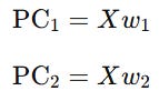
Where each wi maximizes variance and is orthogonal to the previous ones. When your data is a time series (like stock prices, sensor readings, or weather data over time), each time step can be seen as a snapshot of multiple variables. Instead of analyzing each variable separately, PCA lets you:

• Find hidden patterns that combine variables (hot & dry vs. cool & humid patterns).

• Reduce noise.

• Work with fewer features for machine learning.

But why should we use PCA? If you have dozens or hundreds of correlated signals, PCA can shrink it down to a few components. Additionally, components can reveal hidden trends or cycles.

Let’s say you want to predict yt​ (e.g., tomorrow’s temperature) based on many signals.
You could:

• Arrange your data as:

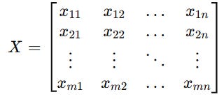
Where each row is a time step, each column is a variable.

• Apply PCA: Keep the top k components that explain most of the variance:

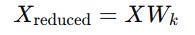
where Wk​ is the matrix of the first k principal component vectors.

• Feed reduced features to your ML model: Use regression on Xreduced​ to predict future values.

If you have 50 stock price time series, they’re probably highly correlated. PCA might reveal that just 3 components explain 90% of the movement.
You can then train your predictive model on those 3 components instead of all 50 prices — less noise, faster training, better generalization.

Do you want to master Deep Learning techniques tailored for time series, trading, and market analysis🔥? My book breaks it all down from basic machine learning to complex multi-period LSTM forecasting while going through concepts such as fractional differentiation and forecasting thresholds. Get your copy here 📖!

---

Introduction to XGBoost

Imagine you’re trying to solve a complex puzzle. Each piece of the puzzle represents a small part of the solution. XGBoost is like having a group of experts, each specializing in a particular type of puzzle piece. They work together to solve the puzzle. The algorithm is all about improving, or boosting, the performance of a model. It starts with a simple model, like a decision tree, and gradually makes it better.

XGBoost pays extreme attention to its mistakes. It looks at the pieces of the puzzle it got wrong and focuses on solving those first. Instead of relying on a single expert to solve the entire puzzle, it uses many experts (decision trees). Each expert gives their opinion on how to solve the puzzle, and they vote together to make the final decision.

XGBoost then goes through a lot of practice puzzles (training data) to train its experts. It learns from its mistakes and gets better over time. It also constantly checks how well it’s doing and makes adjustments. It’s like each expert is given a chance to reevaluate their opinion and improve their piece of the puzzle.

The final solution is the combination of all the expert opinions. This combination often leads to a much better result than just one expert could achieve.

Last year, the development team has been focusing on enhancing XGBoost with vector-leaf tree models for multi-target regression and classification tasks. This new feature allows XGBoost to construct a single tree for all targets, rather than building separate models for each target as it did previously.

This approach brings several advantages and trade-offs compared to the traditional method. It can mitigate overfitting, generate more compact models, and create trees that account for correlations between targets. Additionally, users can incorporate both vector-leaf and scalar-leaf trees in their training sessions using a callback mechanism.

---

Application of the Machine Learning Model

We will simply generate a random walk, apply the PCA algorithm, apply XGBoost forecasting, sum the predictions, and create a full value to predict the original time series.

Use the following code to implement the experiment, knowing that this is just a basic implementation (as many other more complex techniques such as multi-layered forecasting can be applied).

import numpy as np
import matplotlib.pyplot as plt
from sklearn.decomposition import PCA
from xgboost import XGBRegressor

# ---------- Utilities ----------
def create_X_y(series, window_size):
    X, y = [], []
    for i in range(len(series) - window_size):
        X.append(series[i:i+window_size])
        y.append(series[i+window_size])
    return np.array(X), np.array(y)

# ---------- Generate synthetic random walk ----------
np.random.seed(614)
n = 1000
steps = np.random.normal(loc=0, scale=1, size=n)
random_walk = np.cumsum(steps)

# ---------- Make series stationary: first differencing ----------
diff = np.diff(random_walk)          
# Alternative for financial prices: returns = np.diff(np.log(price))

# Forecasting parameters
window_size = 500           # lag embedding window for PCA
comp_window = 100           # window used to model component time-series (can be different)
n_components = 5            # fixed number of PCA components
forecast_horizon = 50       # how many future points to forecast

# ---------- Split: training portion excludes the future horizon ----------
train_diff = diff[:-forecast_horizon]    # only past data used for decomposition & model training
true_future_diff = diff[-forecast_horizon:]  # for plotting/evaluation

# ---------- Build lagged matrix (each row is a window) for PCA ----------
X_lagged_train, _ = create_X_y(train_diff, window_size)  # shape (T_train, window_size)
T_train = X_lagged_train.shape[0]

# ---------- Fit PCA on lagged training windows (no look-ahead) ----------
pca = PCA(n_components=n_components)
components_train = pca.fit_transform(X_lagged_train)  # shape (T_train, n_components)

# ---------- Train one XGB per PCA component using component-time-series ----------
models = []
comp_series = components_train  # each column is a component time series aligned to windows
for c in range(n_components):
    series_c = comp_series[:, c]
    Xc, yc = create_X_y(series_c, comp_window)
    # Use all available Xc,yc for training (we reserved forecast horizon by slicing earlier)
    model = XGBRegressor(n_estimators=100, max_depth=3, verbosity=0)
    model.fit(Xc, yc)
    models.append(model)

# ---------- Recursive multi-step forecasting ----------
# 1) Maintain component-history windows for forecasting (start from last comp windows in training)
comp_histories = [list(comp_series[-comp_window: , c]) for c in range(n_components)]
# 2) Maintain a lagged-window of diffs (last observed window from training), to update by inverse PCA results
last_lagged_window = X_lagged_train[-1].tolist()  # length == window_size

predicted_diff = []       # will collect forecast_horizon predicted differenced values

for t in range(forecast_horizon):
    # Predict each component one step ahead using its own model and history
    next_comp_vals = []
    for c in range(n_components):
        hist = comp_histories[c]
        x_in = np.array(hist[-comp_window:]).reshape(1, -1)
        pred_c = models[c].predict(x_in)[0]
        next_comp_vals.append(pred_c)

    # Convert next component vector to reconstructed lagged features via inverse PCA
    next_comp_vec = np.array(next_comp_vals).reshape(1, -1)   # shape (1, n_components)
    reconstructed_lagged = pca.inverse_transform(next_comp_vec).flatten()  # length == window_size

    # The target next differenced value corresponds to the last element of that reconstructed window
    next_diff = reconstructed_lagged[-1]
    predicted_diff.append(next_diff)

    # Update the lagged window: slide by one, append predicted_diff
    last_lagged_window = last_lagged_window[1:] + [next_diff]

    # Also update each component history to include the newly predicted component (for multi-step recursion)
    for c in range(n_components):
        comp_histories[c].append(next_comp_vals[c])

# ---------- Reconstruct level forecast from differenced forecasts ----------
# Last observed level (price) before the forecast start:
last_observed_level = random_walk[-forecast_horizon-1]  # because diff aligned: diff[-forecast_horizon-1] -> ??? safe choice:
# Simpler: take last known actual level at index n - forecast_horizon - 1
last_observed_level = random_walk[n - forecast_horizon - 1]

forecast_levels = []
current = last_observed_level
for d in predicted_diff:
    current = current + d
    forecast_levels.append(current)

# ---------- Plot ----------
plt.figure(figsize=(12,5))
plt.plot(random_walk, label="Original levels", alpha=0.5)
split_idx = n - forecast_horizon
plt.axvline(split_idx, color='gray', linestyle='--', label='Forecast start')
x_fore = np.arange(split_idx, n)
plt.plot(x_fore, forecast_levels, label="PCA+XGB forecast (levels)", color='red')
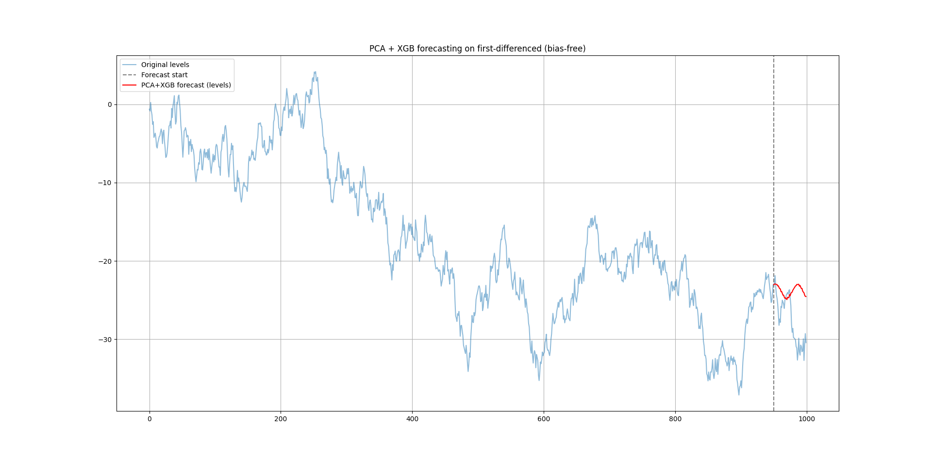
plt.title("PCA + XGB forecasting on first-differenced (bias-free)")
plt.legend()
plt.grid(True)
plt.show()

The following chart shows the output.

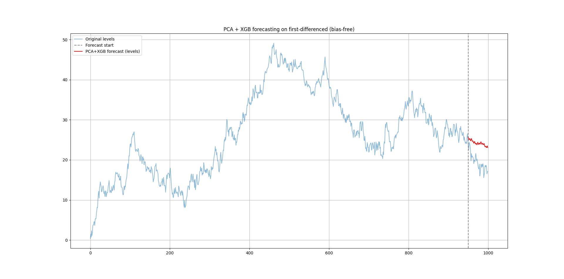
Each value is predicted one step at a time, using the previous prediction as input for the next.

The following chart shows another randomly generated time series with the same experiment (you just need to tweak the random.seed() parameter).

PCA doesn’t predict anything by itself — it transforms your raw time series data into a smaller set of orthogonal signals that make prediction easier for machine learning models.

Every week, I analyze positioning, sentiment, and market structure. Curious what hedge funds, retail, and smart money are doing each week? Then join hundreds of readers here in the Weekly Market Sentiment Report 📜 and stay ahead of the game through chart forecasts, sentiment analysis, volatility diagnosis, and seasonality charts.

Free trial available🆓