
Fibonacci Volatility Bands and Trend Following
The Magic of Trend Following With Volatility Bands

For years, traders have been using volatility bands for contrarian trading but also for trend following. Many types of volatility bands exist such as Bollinger bands, Keltner channel, and Donchian channel. This article will discuss another type of volatility bands called the Fibonacci volatility bands.
A Primer on Volatility Bands
Volatility bands are lines plotted above and below a central price measure (typically a moving average). The distance between the bands and the central line depends on price volatility—when volatility increases, the bands widen; when it decreases, they narrow. The most famous type of volatility bands are Bollinger bands. At their core, Bollinger bands consist of three components:
Middle band – a simple moving average (SMA), usually over 20 periods.
Upper band – the SMA plus 2 standard deviations.
Lower band – the SMA minus 2 standard deviations.
The bands are to be used in the following simple way:
Whenever the price is near upper band, the market is potentially overbought.
Whenever the price is near lower band, the market is potentially oversold.
The following chart shows an example of Bollinger bands.

Fibonacci Volatility Bands
This type of volatility bands was inspired by the Fibonacci moving average, an indicator I have published a few years back. The main idea is to use the Bollinger bands formula on the Fibonacci moving average instead of a simple moving average.
The Fibonacci moving average is calculated as follows:
Calculate different SMAs of the low price using the following lookback periods {5, 8, 13, 21, 34, 55, 89, 144}. After that calculate the difference from the standard deviations of the same source using the same lookback periods.
Calculate different SMAs of the high price using the following lookback periods {5, 8, 13, 21, 34, 55, 89, 144}. After that calculate the difference from the standard deviations of the same source using the same lookback periods.
Calculate the two averages of the two previous steps. The first one will give the Fibonacci’s lower band and the second one will give the upper band.
The following chart shows the Fibonacci volatility bands in action.

They are to be used exactly the same way as Bollinger bands. Mathematically, they will always be wider than the regular 20-period Bollinger bands, and therefore give more breathing space to the market to hover before reaching a crucial inflexion point.
This may make the Fibonacci volatility bands seem to envelop the market better.
In trending markets, you can use the bands to follow the trend every time the price goes back to the lower or upper extreme. The following chart shows the market’s reaction every time it goes back to the lower band during a bullish regime.
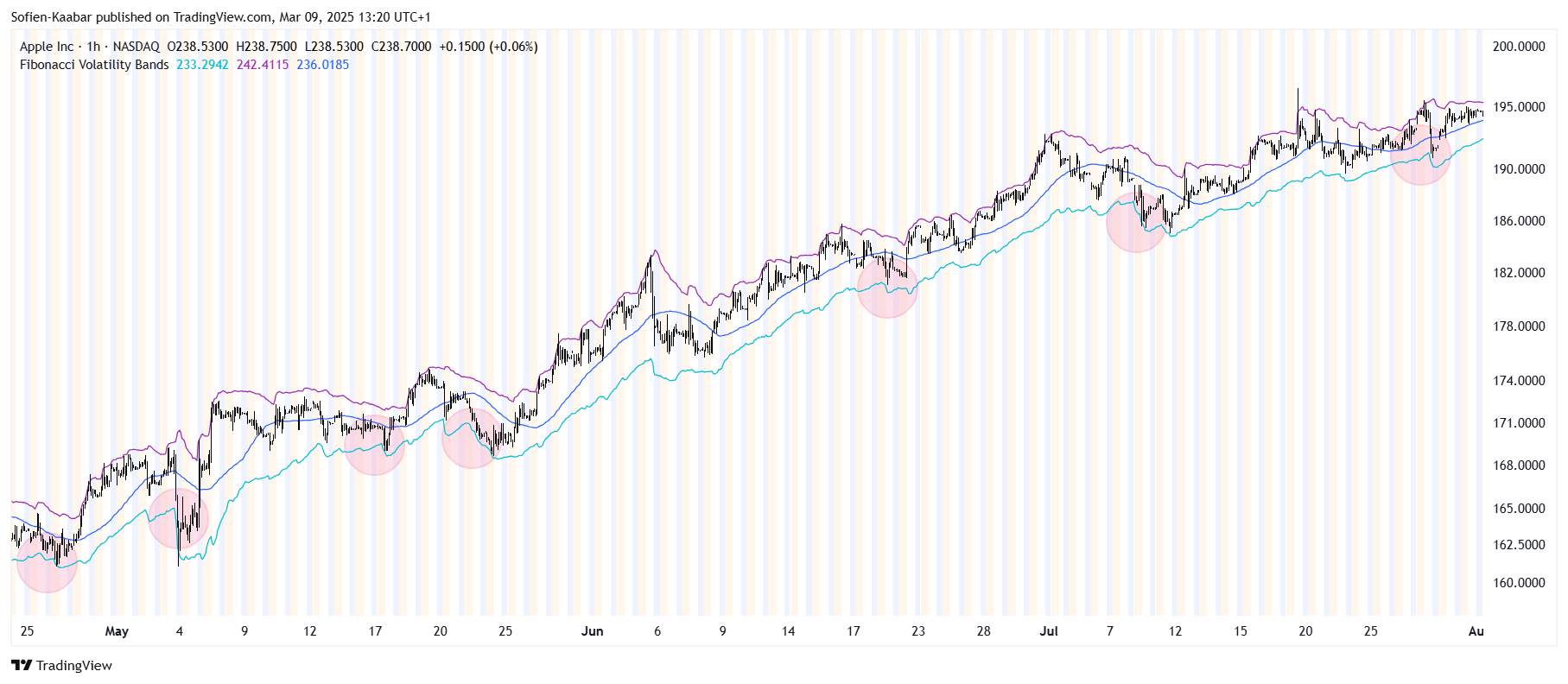
Check out my newsletter that sends weekly directional views every weekend to highlight the important trading opportunities using a mix between sentiment analysis (COT report, put-call ratio, etc.) and rules-based technical analysis.

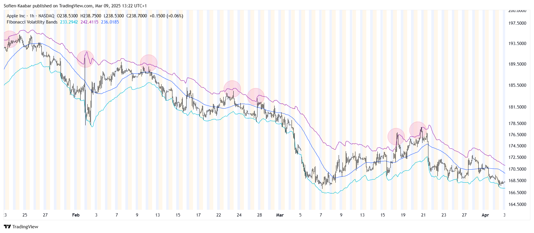
The following chart shows the market’s reaction every time it goes back to the upper band during a bearish regime.
The following code shows how to create the Fibonacci volatility bands in PineScript.
// This source code is subject to the terms of the Mozilla Public License 2.0 at https://mozilla.org/MPL/2.0/
// © Sofien-Kaabar

//@version=5
indicator("Fibonacci Volatility Bands", overlay = true)

first_boll_upper     = ta.sma(high, 5)   + (ta.stdev(high, 5)   * 2)
second_boll_upper    = ta.sma(high, 8)   + (ta.stdev(high, 8)   * 2)
third_boll_upper     = ta.sma(high, 13)  + (ta.stdev(high, 13)  * 2)
fourth_boll_upper    = ta.sma(high, 21)  + (ta.stdev(high, 21)  * 2)
fifth_boll_upper     = ta.sma(high, 34)  + (ta.stdev(high, 34)  * 2)
sixth_boll_upper     = ta.sma(high, 55)  + (ta.stdev(high, 55)  * 2)
seventh_boll_upper   = ta.sma(high, 89)  + (ta.stdev(high, 89)  * 2)
eigth_boll_upper     = ta.sma(high, 144) + (ta.stdev(high, 144) * 2)

av_boll_upper = (first_boll_upper +
           second_boll_upper +
           third_boll_upper +
           fourth_boll_upper +
           fifth_boll_upper +
           sixth_boll_upper +
           seventh_boll_upper +
           eigth_boll_upper) / 8

first_boll_lower     = ta.sma(low, 5)   - (ta.stdev(low, 5)   * 2)
second_boll_lower    = ta.sma(low, 8)   - (ta.stdev(low, 8)   * 2)
third_boll_lower     = ta.sma(low, 13)  - (ta.stdev(low, 13)  * 2)
fourth_boll_lower    = ta.sma(low, 21)  - (ta.stdev(low, 21)  * 2)
fifth_boll_lower     = ta.sma(low, 34)  - (ta.stdev(low, 34)  * 2)
sixth_boll_lower     = ta.sma(low, 55)  - (ta.stdev(low, 55)  * 2)
seventh_boll_lower   = ta.sma(low, 89)  - (ta.stdev(low, 89)  * 2)
eigth_boll_lower     = ta.sma(low, 144) - (ta.stdev(low, 144) * 2)

av_boll_lower = (first_boll_lower +
           second_boll_lower +
           third_boll_lower +
           fourth_boll_lower +
           fifth_boll_lower +
           sixth_boll_lower +
           seventh_boll_lower +
           eigth_boll_lower) / 8

plot(av_boll_lower, color = color.aqua)
plot(av_boll_upper, color = color.purple)
plot(ta.sma(close, 50))
You are advised to use the bands during:
Range-bound markets for mean reversion.
Low volatility periods to anticipate breakouts. You can also use it as an overlay with momentum indicators (like RSI) for stronger signals.