Diversify Your Trading With These Volatility Bands
How to Code & Use the K’s Volatility Bands in Pine Script
The great Bollinger Bands are one of the first things we must learn when analyzing time series. This is because of their sound statistical reasoning, their wide adoption across market participants, and their success when deployed in trading strategies. We can also see other variations that resemble the Bands in an attempt to enhance it. This article will show how to code K’s volatility bands using Pine Script (TradingView’s coding language).
For the complete collection of candlestick patterns in detail with back-tests and technical strategies, you can check out my newest book with O’Reilly Media. The book features a huge number of classic and modern candlestick patterns as it dwelves into the realm of technical analysis with different trading strategies. The book comes with its own GitHub and is dynamic in nature as it is continuously updated and questions are answered on the O’Reilly platform promptly.
Mastering Financial Pattern Recognition
Amazon.com: Mastering Financial Pattern Recognition eBook : Kaabar, Sofien: Kindle Storeamzn.to
K’s Volatility Bands
As stated previously, the volatility bands family contains many indicators which have been discussed in previous articles such as:
The Bollinger bands: These are the pioneers which are predominantly used. They are based on a simple moving average and a standard deviation envelope around the market price.
The augmented Bollinger bands: They try to enhance the previous calculation by including the highs and lows in the calculation and an exponential moving average to take into account more recent data.
The Keltner channel: The channel is calculated using the average true range indicator, a volatility proxy that replaces the standard deviation measure used in the previous two bands.
The VAMA bands: Based on the volatility-adjusted moving average, the VAMA band gives a sizeable weight to volatility so that risk is accounted for. They are the same as the Bollinger bands but simply use the volatility-adjusted moving average instead of the simple one.
The fractal adaptive volatility bands: Also a simple bands overlay indicator based on another type of moving averages called the fractal adaptive moving average.
The aim now is to present another indicator which shares some common traits with the augmented Bollinger bands but takes it to a slightly higher level.
We must first start by calculating a rolling measure based on the average between the highest high and the lowest low in the last specified lookback window.
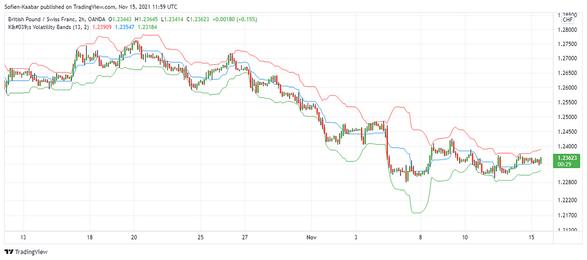
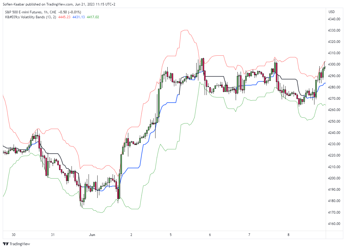
This will give us a type of moving average that tracks the market price. The specificity here is that when the market does not make higher highs nor lower lows, the line will be flat. A flat line can also be thought of as a magnet of the price as the ranging property could hint to a further sideways movement.
The K’s volatility bands assume the worst with volatility and thus will take the maximum volatility for a given lookback period. Unlike the Bollinger bands which will take the latest volatility calculation every single step of time, K’s volatility bands will suppose that we must be protected by the maximum of volatility for that period which will give us from time to time stable support and resistance levels. The formula for the bands can be written down as follows. We can add a multiplier to the formula if we wish.
Coding K’s Volatility Bands in Pine Script
We want to create and plot the K’s volatility bands on the GBPCHF values loaded on the TradingView platform. Note that you must create an account to be able to view the charts, the good news is that it is free. Locate the Chart button on the home screen and then choose any asset you would like to calculate the indicator on. Now, on the bottom of the screen, locate Pine Editor and warm up your fingers to do some coding.
//@version = 5The next step is to specify the name of the indicator by using the following syntax. We must also set the overlay argument to true because we want to chart the bands in the same panel as the price. Setting it to false will put the bands in another panel which makes it difficult to analyze.
indicator("K's Volatility Bands", overlay = true)We can now set the default lookback period values and the multiplier using the input() function.
lookback = input(defval = 13, title = 'Lookback')
multiplier = input(defval = 2, title = 'Multiplier')
Now, we apply the median function using the ta.highest() and ta.lowest() functions which output the highest or lowest values given an array of values and a moving window which basically the lookback period.
median = (ta.highest(high, lookback) + ta.lowest(low, lookback)) / 2The maximum volatility is calculated using the standard deviation function ta.stdev() inside a ta.highest() function so that it outputs the desired result.
maximum_volatility = ta.highest(ta.stdev(close, lookback), lookback)Finally, the bands can be easily calculated following this below syntax.
upper_band = median + (multiplier * maximum_volatility)
lower_band = median - (multiplier * maximum_volatility)
Let us plot the indicator and visualize the chart.
plot(upper_band, color = color.red)
plot(median, color = color.blue)
plot(lower_band, color = color.green)


