Detecting Chart Patterns with Numerical Templates and a Random Walk Price Series

A Practical, Intuition-First Guide With a Python Example

This post walks through a simple, fully controlled setup for detecting chart patterns in a price series without relying on any specialized backtesting framework. The goal is to make the mechanics explicit:

1. Represent chart patterns as numerical sequences

2. Generate a realistic synthetic price series

3. Scan the series for approximate matches using a similarity measure

4. Visualize where those patterns occur

There is no claim here about predictive power. This is about structure and implementation.

---

Representing chart patterns as sequences

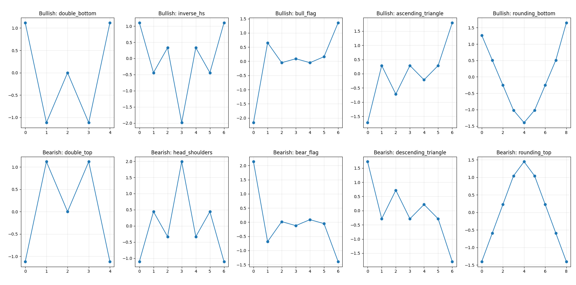
A chart pattern can be reduced to a sequence of relative values. The absolute numbers do not matter. What matters is the shape.

For example:

• A double top can be written as [1, 5, 3, 5, 1]

• A double bottom is simply the inverse: [5, 1, 3, 1, 5]

These sequences encode:

• turning points

• relative height differences

• approximate symmetry

The spacing between elements implicitly represents time. We assume equal spacing for simplicity. Below are the templates used.

Bullish patterns

BULLISH_PATTERNS = {
    "double_bottom":        [5, 1, 3, 1, 5],
    "inverse_hs":           [5, 3, 4, 1, 4, 3, 5],
    "bull_flag":            [1, 5, 4, 4.2, 4.0, 4.3, 6],
    "ascending_triangle":   [2, 4, 3, 4, 3.5, 4, 5.5],
    "rounding_bottom":      [5, 4, 3, 2, 1.5, 2, 3, 4, 5.5],
}

Bearish patterns

BEARISH_PATTERNS = {
    "double_top":           [1, 5, 3, 5, 1],
    "head_shoulders":       [1, 3, 2, 5, 2, 3, 1],
    "bear_flag":            [6, 2, 3, 2.8, 3.1, 2.9, 1],
    "descending_triangle":  [5, 3, 4, 3, 3.5, 3, 1.5],
    "rounding_top":         [1, 2, 3, 4, 4.5, 4, 3, 2, 1],
}

These are not precise definitions. They are rough templates that capture the intended geometry.

---

Generating a realistic price series

To test pattern detection properly, the data should not contain obvious structure. A sine wave or deterministic trend makes the problem trivial.

Instead, we simulate a geometric random walk with volatility clustering, which is closer to financial time series.

np.random.seed(7)
n = 700
dates = pd.date_range("2022-01-01", periods=n, freq="D")
omega = 0.000005
alpha = 0.05
beta = 0.9
returns = np.zeros(n)
variance = np.zeros(n)
variance[0] = 0.0001
for t in range(1, n):
    variance[t] = omega + alpha * (returns[t-1]**2) + beta * variance[t-1]
    returns[t] = np.random.normal(0, np.sqrt(variance[t]))
drift = 0.0002
returns = returns + drift
price = 100 * np.exp(np.cumsum(returns))
price = pd.Series(price, index=dates, name="Close")

Key properties of this process:

• Prices evolve multiplicatively (log returns)

• Volatility changes over time

• There is no embedded pattern by construction

This makes any detected pattern the result of coincidence or genuine structure in the algorithm, not in the data generation.

I started Quant Atlas, a platform for Quantitative forecasting through charts, powered by multiple models working together. 📈

No noise. No guesswork. Just structured, data-driven market forecasts across assets.

If you want to see how it actually performs in real time, you can try it yourself.

Comparing Price Windows to Pattern Templates

We now need a way to compare a segment of the price series to a pattern. There are two issues:

1. The window and the pattern may have different lengths

2. Absolute price levels are irrelevant

Step 1: resample to the same length

Each rolling window is interpolated to match the number of points in the pattern.

def resample_to_length(x, target_len):
    old_idx = np.linspace(0, 1, len(x))
    new_idx = np.linspace(0, 1, target_len)
    return np.interp(new_idx, old_idx, x)

Step 2: normalize

We remove scale and location using z-score normalization:

def zscore(x):
    std = np.std(x)
    if std < 1e-12:
        return np.zeros_like(x)
    return (x - np.mean(x)) / std

Step 3: compute distance

We measure similarity using root mean squared error:

def pattern_distance(window, pattern):
    window_rs = resample_to_length(window, len(pattern))
    w = zscore(window_rs)
    p = zscore(pattern)
    return np.sqrt(np.mean((w - p) ** 2))

A smaller distance means a closer match in shape.

---

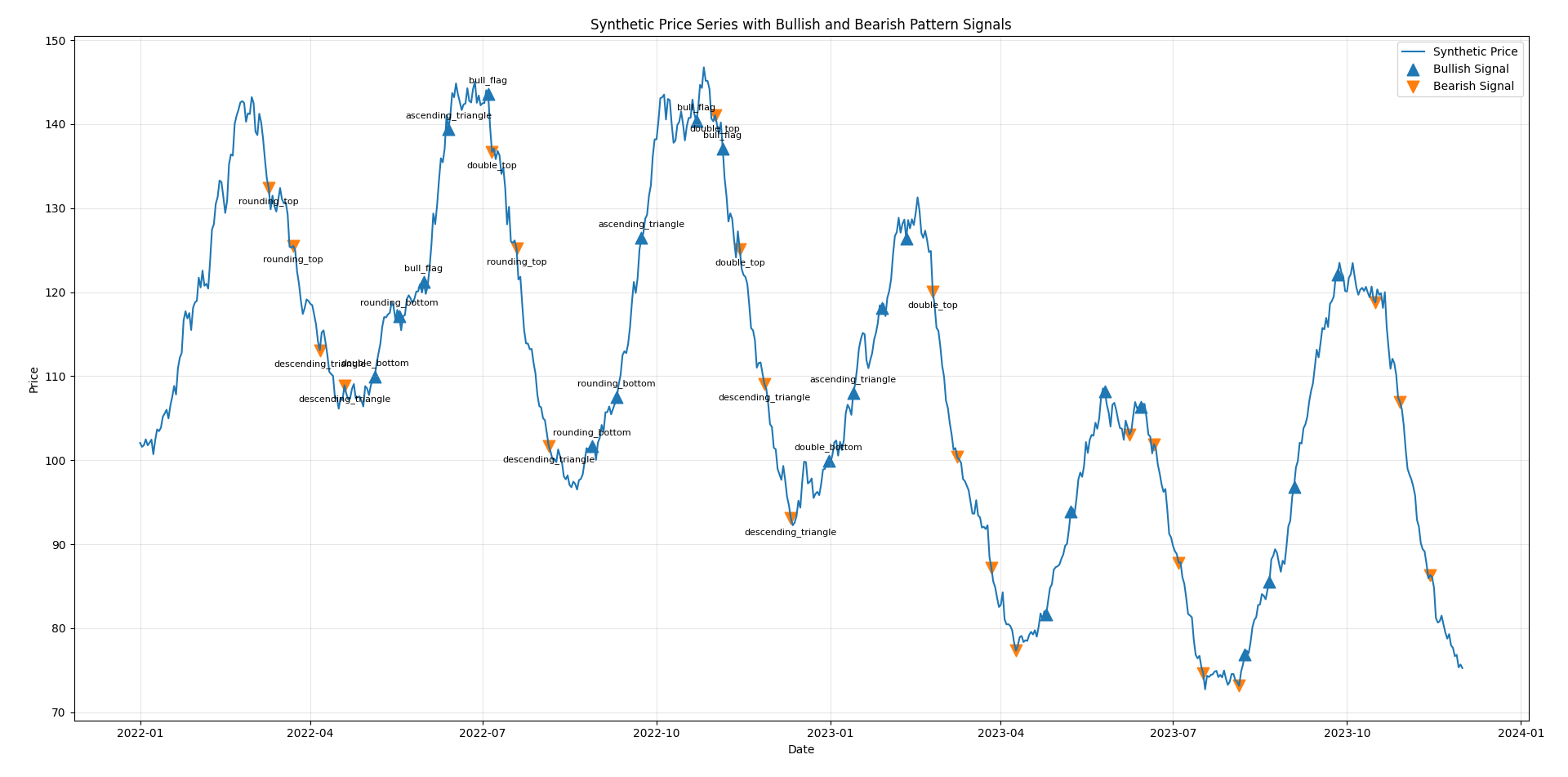
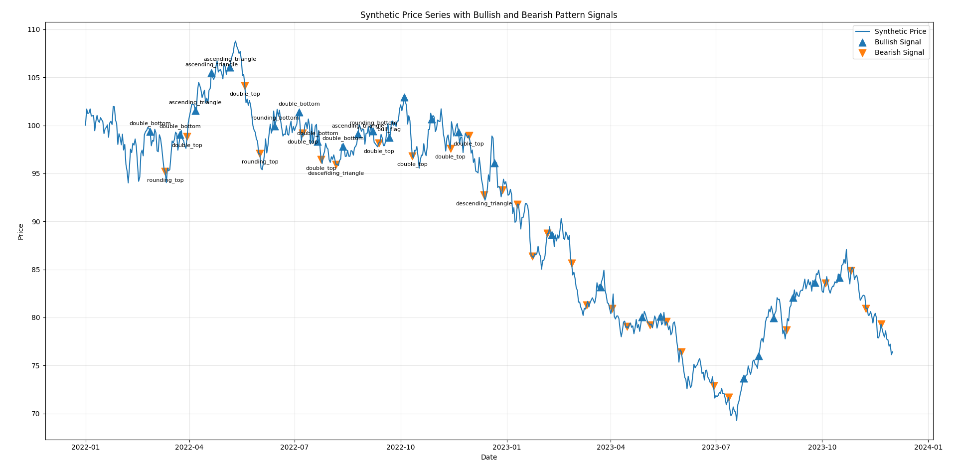
Scanning the Time Series

We slide a window across the price series and compare each segment to all pattern templates. For each time step:

• evaluate multiple window sizes

• compute distance to each pattern

• keep the best match

If the best match is below a threshold, we emit a signal.

WINDOW_SIZES = [24, 32, 40, 48, 56]
THRESHOLD = 0.62
COOLDOWN_BARS = 12

• Window sizes allow flexibility in pattern duration

• Threshold controls strictness

• Cooldown prevents repeated signals in a short span

This produces two time series:

• bullish signals

• bearish signals

Each signal is also labeled with the matched pattern.

---

What the algorithm is actually doing

At each time t, the algorithm answers:

Does the recent price path look like any of these templates?

It does not:

• forecast future returns

• optimize parameters

• evaluate profitability

It is purely a shape-matching procedure. Because of normalization, it is invariant to:

• scale (price level)

• amplitude (volatility)

Because of resampling, it is tolerant to:

• different durations

• slight distortions

---

Visualization

The final output is a price chart with markers:

• upward triangles for bullish matches

• downward triangles for bearish matches

Each marker corresponds to the end of a window that matched a pattern. In practice, you will observe:

• clusters of signals during volatile periods

• occasional overlapping bullish and bearish matches

• many imperfect matches (as expected)

This reflects the fact that the underlying data is largely random.

import numpy as np
import pandas as pd
import matplotlib.pyplot as plt

BULLISH_PATTERNS = {
    "double_bottom":        [5, 1, 3, 1, 5],
    "inverse_hs":           [5, 3, 4, 1, 4, 3, 5],   # inverse head & shoulders
    "bull_flag":            [1, 5, 4, 4.2, 4.0, 4.3, 6],
    "ascending_triangle":   [2, 4, 3, 4, 3.5, 4, 5.5],
    "rounding_bottom":      [5, 4, 3, 2, 1.5, 2, 3, 4, 5.5],
}

BEARISH_PATTERNS = {
    "double_top":           [1, 5, 3, 5, 1],
    "head_shoulders":       [1, 3, 2, 5, 2, 3, 1],
    "bear_flag":            [6, 2, 3, 2.8, 3.1, 2.9, 1],
    "descending_triangle":  [5, 3, 4, 3, 3.5, 3, 1.5],
    "rounding_top":         [1, 2, 3, 4, 4.5, 4, 3, 2, 1],
}

ALL_PATTERNS = {**BULLISH_PATTERNS, **BEARISH_PATTERNS}

def zscore(x):
    x = np.asarray(x, dtype=float)
    std = np.std(x)
    if std < 1e-12:
        return np.zeros_like(x)
    return (x - np.mean(x)) / std

def resample_to_length(x, target_len):
    """
    Linearly resample a 1D array to target_len points.
    """
    x = np.asarray(x, dtype=float)
    old_idx = np.linspace(0, 1, len(x))
    new_idx = np.linspace(0, 1, target_len)
    return np.interp(new_idx, old_idx, x)

def pattern_distance(window, pattern):
    """
    Compare a rolling price window to a pattern template.
    Both are resampled to the same length and z-scored.
    Lower distance = better match.
    """
    pattern = np.asarray(pattern, dtype=float)
    window_rs = resample_to_length(window, len(pattern))
    w = zscore(window_rs)
    p = zscore(pattern)
    return np.sqrt(np.mean((w - p) ** 2))

np.random.seed(7)

n = 700
dates = pd.date_range("2022-01-01", periods=n, freq="D")

# --- GARCH-like volatility clustering (simple version) ---
omega = 0.000005
alpha = 0.05
beta = 0.9

returns = np.zeros(n)
variance = np.zeros(n)

variance[0] = 0.0001

for t in range(1, n):
    variance[t] = omega + alpha * (returns[t-1]**2) + beta * variance[t-1]
    returns[t] = np.random.normal(0, np.sqrt(variance[t]))

# small drift (realistic)
drift = 0.0002
returns = returns + drift

# geometric random walk
price = 100 * np.exp(np.cumsum(returns))
price = pd.Series(price, index=dates, name="Close")

WINDOW_SIZES = [24, 32, 40, 48, 56]
THRESHOLD = 0.62         # lower = stricter matching
COOLDOWN_BARS = 12       # suppress repeated nearby signals

bullish_signal = pd.Series(False, index=price.index)
bearish_signal = pd.Series(False, index=price.index)

bullish_label = pd.Series("", index=price.index, dtype="object")
bearish_label = pd.Series("", index=price.index, dtype="object")

last_bull_idx = -10_000
last_bear_idx = -10_000

values = price.values

for i in range(max(WINDOW_SIZES), len(price)):
    best_bull_dist = np.inf
    best_bull_name = None

    best_bear_dist = np.inf
    best_bear_name = None

    # Search over multiple window lengths and all templates
    for w in WINDOW_SIZES:
        window = values[i - w:i]

        for name, pattern in BULLISH_PATTERNS.items():
            dist = pattern_distance(window, pattern)
            if dist < best_bull_dist:
                best_bull_dist = dist
                best_bull_name = name

        for name, pattern in BEARISH_PATTERNS.items():
            dist = pattern_distance(window, pattern)
            if dist < best_bear_dist:
                best_bear_dist = dist
                best_bear_name = name

    # Emit bullish signal
    if best_bull_dist < THRESHOLD and (i - last_bull_idx) > COOLDOWN_BARS:
        bullish_signal.iloc[i] = True
        bullish_label.iloc[i] = best_bull_name
        last_bull_idx = i

    # Emit bearish signal
    if best_bear_dist < THRESHOLD and (i - last_bear_idx) > COOLDOWN_BARS:
        bearish_signal.iloc[i] = True
        bearish_label.iloc[i] = best_bear_name
        last_bear_idx = i

# Optional conflict cleanup:
# if both happen on same bar, keep only the better one
same_bar = bullish_signal & bearish_signal
for idx in np.where(same_bar)[0]:
    i = idx
    best_bull_dist = np.inf
    best_bear_dist = np.inf
    for w in WINDOW_SIZES:
        if i - w < 0:
            continue
        window = values[i - w:i]
        for pattern in BULLISH_PATTERNS.values():
            best_bull_dist = min(best_bull_dist, pattern_distance(window, pattern))
        for pattern in BEARISH_PATTERNS.values():
            best_bear_dist = min(best_bear_dist, pattern_distance(window, pattern))
    if best_bull_dist <= best_bear_dist:
        bearish_signal.iloc[i] = False
        bearish_label.iloc[i] = ""
    else:
        bullish_signal.iloc[i] = False
        bullish_label.iloc[i] = ""

signals = pd.DataFrame({
    "price": price,
    "bullish_signal": bullish_signal,
    "bullish_pattern": bullish_label,
    "bearish_signal": bearish_signal,
    "bearish_pattern": bearish_label
})

print("\nDetected bullish signals:")
print(signals.loc[signals["bullish_signal"], ["price", "bullish_pattern"]].head(20))

print("\nDetected bearish signals:")
print(signals.loc[signals["bearish_signal"], ["price", "bearish_pattern"]].head(20))

plt.figure(figsize=(15, 8))
plt.plot(price.index, price.values, label="Synthetic Price", linewidth=1.5)

bull_idx = bullish_signal[bullish_signal].index
bear_idx = bearish_signal[bearish_signal].index

plt.scatter(
    bull_idx,
    price.loc[bull_idx],
    marker="^",
    s=110,
    label="Bullish Signal"
)

plt.scatter(
    bear_idx,
    price.loc[bear_idx],
    marker="v",
    s=110,
    label="Bearish Signal"
)

# Annotate a subset to keep the chart readable
for dt in bull_idx[:12]:
    plt.annotate(
        bullish_label.loc[dt],
        (dt, price.loc[dt]),
        xytext=(0, 10),
        textcoords="offset points",
        ha="center",
        fontsize=8
    )

for dt in bear_idx[:12]:
    plt.annotate(
        bearish_label.loc[dt],
        (dt, price.loc[dt]),
        xytext=(0, -14),
        textcoords="offset points",
        ha="center",
        fontsize=8
    )

plt.title("Synthetic Price Series with Bullish and Bearish Pattern Signals")
plt.xlabel("Date")
plt.ylabel("Price")
plt.legend()
plt.grid(True, alpha=0.3)
plt.tight_layout()
plt.show()

fig, axes = plt.subplots(2, 5, figsize=(16, 6))

for ax, (name, pattern) in zip(axes[0], BULLISH_PATTERNS.items()):
    ax.plot(zscore(pattern), marker="o")
    ax.set_title(f"Bullish: {name}")
    ax.grid(True, alpha=0.3)

for ax, (name, pattern) in zip(axes[1], BEARISH_PATTERNS.items()):
    ax.plot(zscore(pattern), marker="o")
    ax.set_title(f"Bearish: {name}")
    ax.grid(True, alpha=0.3)

plt.tight_layout()
plt.show()

This approach is intentionally simple. Its limitations are clear:

• No notion of trend context

• No volume or multi-dimensional input

• No statistical validation

• High sensitivity to threshold choice

Most importantly:

Pattern detection does not imply predictive value.

On a random walk, patterns will still appear. This is a direct consequence of randomness and finite samples.

Despite its simplicity, this framework is useful for:

• Prototyping pattern definitions

• Testing robustness of pattern detection

• Understanding how often patterns occur by chance

• Building intuition before introducing more complex models

The entire pipeline is deliberately explicit:

• patterns are defined as sequences

• similarity is defined mathematically

• detection is a sliding-window search

There are no hidden components. If the algorithm produces signals, you can trace exactly why. That clarity is the main advantage of building it this way.