Create a Time-Based Technical Trading Strategy.
Creating a Trading Strategy Based on Temporal Analysis.
Temporal analysis is related to the concept of time. In technical analysis, we are often more concerned with levels and how extreme they regarding normality. In this article, we will try to elaborate a simple idea that is based on both time and extreme readings on technical indicators so that we see whether it offers quality signals or not. We will create the indicator, formulate the strategy, and then evaluate it.
I have just released a new book after the success of the previous book. It features advanced trend following indicators and strategies with a GitHub page dedicated to the continuously updated code. Also, this book features the original colors after having optimized for printing costs. If you feel that this interests you, feel free to visit the below Amazon link, or if you prefer to buy the PDF version, you could contact me on LinkedIn.
The Trend Intensity Index
The trend intensity index is a measure of the strength of the trend. It is a relatively simple calculation to make. The indicator is created by a 10-period moving average and price deviations around it, then, we will count the number of the up periods relative to the total number of periods. Let us build the indicator step-by-step:
Define the lookback period which is set at 10 and calculate the moving average on the market price using this lookback period.
lookback = 10# Defining the Primal Manipulation Functions
def adder(Data, times):
for i in range(1, times + 1):
new = np.zeros((len(Data), 1), dtype = float)
Data = np.append(Data, new, axis = 1) return Datadef deleter(Data, index, times):
for i in range(1, times + 1):
Data = np.delete(Data, index, axis = 1)return Data
def jump(Data, jump):
Data = Data[jump:, ]
return Data# Defining the Moving Average Function
def ma(Data, lookback, close, where):
Data = adder(Data, 1)
for i in range(len(Data)):
try:
Data[i, where] = (Data[i - lookback + 1:i + 1, close].mean())
except IndexError:
pass
# Cleaning
Data = jump(Data, lookback)
return Data# Calculating the Moving Average
Data = ma(my_data, lookback, 3, 4)# Note that for the code to work properly, you need to have an OHLC historical data in the form of a numpy arrayCalculate the deviations of the market price from the moving average. This is done by doing so on two columns. If the current market price is greater than its 10-period moving average, then the first column will be filled by the difference between the two (Market price minus moving average). If the current market price is lower than its 10-period moving average, then the second column will be filled by the difference between the two (Moving average minus market price).
# Deviations
for i in range(len(my_data)):

   if my_data[i, what] > my_data[i, where]:
      my_data[i, where + 1] = my_data[i, what] - my_data[i, where]

   if my_data[i, what] < my_data[i, where]:
      my_data[i, where + 2] = my_data[i, where] - my_data[i, what]
Now, we want to count the values where the market was above its 10-period moving average and where it was below it. This can be done using the numpy function count_nonzero():
for i in range(len(Data)):

  Data[i, where + 3] = np.count_nonzero(Data[i - lookback + 1:i + 1, where + 1])

for i in range(len(Data)):

  Data[i, where + 4] = np.count_nonzero(Data[i - lookback + 1:i + 1, where + 2])
And finally, we can calculate the Trend Intensity Index using the below formula with the Python code below it:
# Trend Intensity Index
for i in range(len(Data)):

Data[i, where + 5] = ((Data[i, where + 3]) / (Data[i, where + 3] + Data[i, where + 4])) * 100The code summed up in a function can be written down as follows:
def trend_intensity_index(data, lookback, close, where):

    # Calculating the Moving Average
    data = ma(data, lookback, close, where)
data = adder(data, 5)
# Deviations
for i in range(len(data)):
if data[i, close] > data[i, where]:
data[i, where + 1] = data[i, close] - data[i, where]
if data[i, close] < data[i, where]:
data[i, where + 2] = data[i, where] - data[i, close]
# Trend Intensity Index
for i in range(len(data)):
data[i, where + 3] = np.count_nonzero(data[i - lookback + 1:i + 1, where + 1])
for i in range(len(data)):
data[i, where + 4] = np.count_nonzero(data[i - lookback + 1:i + 1, where + 2])
for i in range(len(data)):
data[i, where + 5] = ((data[i, where + 3]) / (data[i, where + 3] + data[i, where + 4])) * 100
data = deleter(data, where, 5)
return dataThe Duration Strategy
We understand that by looking at the structure of the trend intensity index:
An oversold reading lies at 0 and is saying that the bearish momentum should fade soon and we might see a correction or even a reversal on the upside.
An overbought reading lies at 100 and is saying that the bullish momentum should fade soon and we might see a correction or even a reversal on the downside.
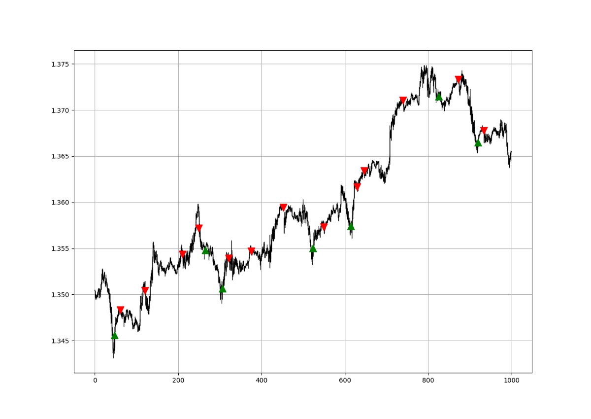
However, if things were so simple, we would all be millionnaires. Our aim from the temporal analysis is to calculate the average time the indicator has spent in the extremes, thus benefitting from both the extreme and time in order to generate a signal. Below is a chart that illustrates this more clearly. For the remainder of the article, we will be using a 3-period trend intensity index.
The above chart shows the EURUSD with the number of periods where the 3-period Trend Intensity Index has been in the extreme zone. A value of -3 means that the index lasted 3 time periods in the zero level. To calculate the Duration, we can follow the below steps:
# Defining the lookback period
lookback = 3
# Calculate the TII on OHLC array (composed of 4 columns)
my_data = trend_intensity_indicator(my_data, lookback, 3, 5)# Add a few spare columns to be populated with whatever you want
my_data = adder(my_data, 20)# Define the Barriers (Oversold and Overbought zones)
upper_barrier = 3
lower_barrier = -3# Define the Extreme Duration
def extreme_duration(Data, indicator, upper_barrier, lower_barrier, where_upward_extreme, where_downward_extreme):
# Time Spent Overbought
for i in range(len(Data)):
if Data[i, indicator] == upper_barrier:
Data[i, where_upward_extreme] = Data[i - 1, where_upward_extreme] + 1
else:
a = 0
Data[i, where_upward_extreme] = a
# Time Spent Oversold
for i in range(len(Data)):
if Data[i, indicator] == lower_barrier:
Data[i, where_downward_extreme] = Data[i - 1, where_downward_extreme] + 1
else:
a = 0
Data[i, where_downward_extreme] = a
Data[:, where_downward_extreme] = -1 * Data[:, where_downward_extreme]
return Datamy_data = adder(my_data, 10)my_data = extreme_duration(my_data, 4, 100, 0, 7, 6)my_data[:, 8] = my_data[:, 6] + my_data[:, 7]Whenever the extreme duration enters the zone between -3/-5 or 3/5, we can say that there will likely be a reaction in the market.
def signal(Data, what, buy, sell):

    Data = adder(Data, 10)

    for i in range(len(Data)):

        if Data[i, what] <= -3 and Data[i - 1, buy] == 0 and \
            Data[i - 2, buy] == 0 and Data[i - 3, buy] == 0 and Data[i - 4, buy] == 0:
            Data[i, buy] = 1

        elif Data[i, what] >= 3 and Data[i - 1, sell] == 0 and \
            Data[i - 2, sell] == 0 and Data[i - 3, sell] == 0 and Data[i - 4, sell] == 0:
            Data[i, sell] = -1

return DataA lot of optimization can be done on this promising technique, especially that only value-wise readings are not sufficient anymore. Temporal analysis is paramount to better understand how the underlying reacts.
If you are also interested by more technical indicators and strategies, then my book might interest you:
Evaluating the Signals
Having had the signals, we now know when the algorithm would have placed its buy and sell orders, meaning, that we have an approximate replica of the past where can can control our decisions with no hindsight bias. We have to simulate how the strategy would have done given our conditions.
This means that we need to calculate the returns and analyze the performance metrics. Let us see what we get if we trade on every signal and close at the next signal.
The hit ratio is 54.00% which means that on 100 trades, we tend to see in 54 of the cases a profitable trade when closing not counting transaction costs. This shows that the strategy on hourly data of the EURUSD since 2011 (~ 932 trades) is not very predictive. The same job must be done on other pairs and other assets to have a full idea on the quality of the strategy. The risk-reward ratio is 0.89 and the profit factor is 1.03 making this a meh strategy at best.
Remember to always do your back-tests. You should always believe that other people are wrong. My indicators and style of trading may work for me but maybe not for you.
I am a firm believer of not spoon-feeding. I have learnt by doing and not by copying. You should get the idea, the function, the intuition, the conditions of the strategy, and then elaborate (an even better) one yourself so that you back-test and improve it before deciding to take it live or to eliminate it. My choice of not providing specific Back-testing results should lead the reader to explore more herself the strategy and work on it more.
One Last Word
I have recently started an NFT collection that aims to support different humanitarian and medical causes. The Society of Light is a set of limited collectibles which will help make the world slightly better as each sale will see a percentage of it sent directly to the charity attributed to the avatar. As I always say, nothing better than a bullet list to outline the benefits of buying these NFT’s:
High-potential gain: By concentrating the remaining sales proceedings on marketing and promoting The Society of Light, I am aiming to maximize their value as much as possible in the secondary market. Remember that trading in the secondary market also means that a portion of royalties will be donated to the same charity.
Art collection and portfolio diversification: Having a collection of avatars that symbolize good deeds is truly satisfying. Investing does not need to only have selfish needs even though there is nothing wrong with investing to make money. But what about investing to make money, help others, and collect art?
Donating to your preferred cause(s): This is a flexible way of allocating different funds to your charities.
A free copy of my book in PDF: Any buyer of any NFT will receive a free copy of my latest book shown in the link of the article.


