Cracking The Dark Pool: Forecasting S&P 500 Using Machine Learning
Creating a Random Forest Algorithm to Predict S&P 500 Returns
Dark pools, also known as alternative trading systems, are private, off-exchange platforms used by institutional investors and high-frequency traders to execute large block orders of stocks and other securities. Unlike traditional stock exchanges, dark pools do not display order book information or the identities of trading participants to the public.
This article will download historical values relating to dark pool activities and will develop a random forest model that aims to predict the returns of the S&P 500 using the dark pool values.
The Dark Index
The dark index (DIX) provides a way of peeking into the secret (dark) exchanges. it is calculated as an aggregate value of many dark pool indicators and measures the hidden market sentiment. When the values of this indicator are higher than usual, it means that more buying occurred in dark pools than usual. We can profit from this informational gap. It is therefore a trail of liquidity providers (i.e. negatively correlated with the market it follows due to hedging activities).
The following graph shows the historical values of the DIX.
The DIX is published on a regular basis by squeezemetrics and is free for download.
Creating the Algorithm
Our aim is to use the values of the index as inputs to feed a random forest algorithm and fit it to the returns of the S&P 500 index. In layman’s terms, we will be creating a machine learning algorithm that uses the index to predict the upcoming S&P 500’s direction (up or down). Here’s the breakdown of the steps:
Pip install selenium and then download Chrome Webdriver (make sure that it is compatible with your Google Chrome version).
Use the script provided below to download automatically the historical values of the index and the S&P 500. Take the returns and shift the values of the index by a number of lags (in this case, 34).
Clean the data and split it into test and training data.
Fit and predict using the random forest regression algorithm.
Evaluate the results using the hit ratio (accuracy).
✨ Important note
Note: The index is stationary. This means that it does not have a trending nature that makes it not suitable for regression.
Use the following code to implement the research:
# Importing Libraries
import pandas as pd
import numpy  as np
from selenium import webdriver
from selenium.webdriver.common.by import By
from sklearn.ensemble import RandomForestRegressor
import matplotlib.pyplot as plt

# Calling Chrome
driver = webdriver.Chrome()
# URL of the Website from Where to Download the Data
url = "https://squeezemetrics.com/monitor/dix"

# Opening the website
driver.get(url)

# Getting the button by ID
button = driver.find_element(By.ID, "fileRequest")
# Clicking on the button
button.click()
# Importing the Excel File Using pandas
my_data = pd.read_csv('DIX.csv')
# Transforming the File to an Array
selected_columns = ['price', 'dix']
my_data = my_data[selected_columns]
my_data['dix'] = my_data['dix'].shift(20)
my_data = my_data.dropna()
my_data = np.array(my_data)
from statsmodels.tsa.stattools import adfuller
print('p-value: %f' % adfuller(my_data[:, 1])[1])
my_data = pd.DataFrame(my_data)
my_data = my_data.diff()
my_data = my_data.dropna()
my_data = np.array(my_data)
def data_preprocessing(data, train_test_split):
    # Split the data into training and testing sets
    split_index = int(train_test_split * len(data))
    x_train = data[:split_index, 1]
    y_train = data[:split_index, 0]
    x_test = data[split_index:, 1]
    y_test = data[split_index:, 0]

    return x_train, y_train, x_test, y_test
x_train, y_train, x_test, y_test = data_preprocessing(my_data, 0.80)
model_rf = RandomForestRegressor(max_depth = 50, random_state = 0)
x_train = np.reshape(x_train, (-1, 1))
x_test = np.reshape(x_test, (-1, 1))
model_rf.fit(x_train, y_train)
y_pred_rf = model_rf.predict(x_test)
same_sign_count_rf = np.sum(np.sign(y_pred_rf) == np.sign(y_test)) / len(y_test) * 100
print('Hit Ratio RF = ', same_sign_count_rf, '%')
plt.plot(y_pred_rf[-100:], label='Predicted Data', linestyle='--', marker = '.', color = 'blue')
plt.plot(y_test[-100:], label='True Data', marker = '.', alpha = 0.7, color = 'red')
plt.legend()
plt.grid()
plt.axhline(y = 0, color = 'black', linestyle = '--')
✨ Important note
Make sure to pip install selenium.
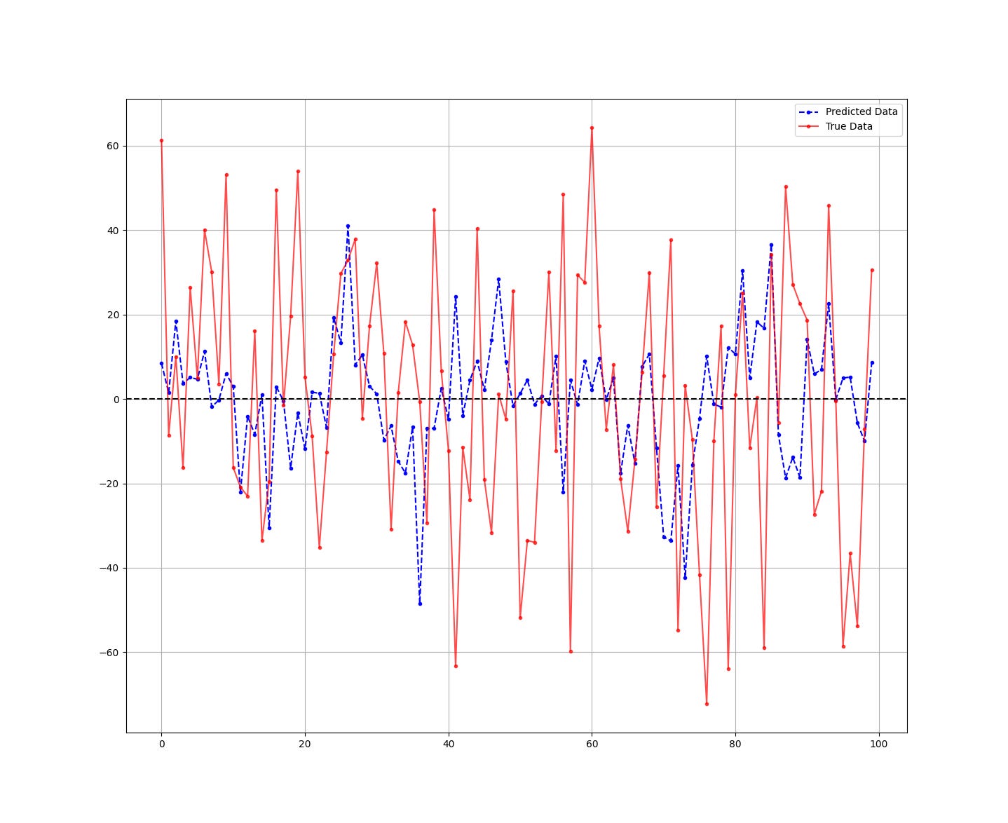
The following Figure compares the predicted (blue) versus the real data (red).
The hit ratio (accuracy) of the algorithm is as follows:
Hit Ratio RF = 52.56 %It seems that the algorithm has had a 52.56% accuracy in determining whether the S&P 500 index will close in the positive or negative territory.
Strangely enough, it had a better forecasting ability with the short predictions than the long ones for a market that has a huge bullish bias.
You can try adding more inputs and tuning the hyperparameters of the algorithm so that the performance gets even better.
You can also check out my other newsletter The Weekly Market Sentiment Report that sends weekly directional views every weekend to highlight the important trading opportunities using a mix between sentiment analysis (COT report, put-call ratio, etc.) and rules-based technical analysis.
If you liked this article, do not hesitate to like and comment, to further the discussion!


