


Combining the Volatility Moving Average With the SuperTrend.
Creating a Strategy Based on the Volatility Moving Average & the SuperTrend.


Combining indicators can be a powerful way to improve performance and to enhance the signals. This article discusses a discretionary strategy which deals with the SuperTrend and the volatility-adjusted moving average to generate trend following signals.
I have just released a new book after the success of my previous one “The Book of Trading Strategies”. It features advanced trend-following indicators and strategies with a GitHub page dedicated to the continuously updated code. Also, this book features the original colors after having optimized for printing costs. If you feel that this interests you, feel free to visit the below Amazon link, or if you prefer to buy the PDF version, you could contact me on LinkedIn.
The Volatility-Adjusted Moving Average
Moving averages help us confirm and ride the trend. They are the most known technical indicator and this is because of their simplicity and their proven track record of adding value to the analyses. We can use them to find support and resistance levels, stops and targets, and to understand the underlying trend. This versatility makes them an indispensable tool in our trading arsenal.
# The function to add a number of columns inside an array
def adder(Data, times):

    for i in range(1, times + 1):

        new_col = np.zeros((len(Data), 1), dtype = float)
        Data = np.append(Data, new_col, axis = 1)

    return Data

# The function to delete a number of columns starting from an index
def deleter(Data, index, times):

    for i in range(1, times + 1):

        Data = np.delete(Data, index, axis = 1)

    return Data

# The function to delete a number of rows from the beginning
def jump(Data, jump):

    Data = Data[jump:, ]

    return Data

# Example of adding 3 empty columns to an array
my_ohlc_array = adder(my_ohlc_array, 3)

# Example of deleting the 2 columns after the column indexed at 3
my_ohlc_array = deleter(my_ohlc_array, 3, 2)

# Example of deleting the first 20 rows
my_ohlc_array = jump(my_ohlc_array, 20)

# Remember, OHLC is an abbreviation of Open, High, Low, and Close and it refers to the standard historical data file

def ma(Data, lookback, close, where):

    Data = adder(Data, 1)

    for i in range(len(Data)):

            try:
                Data[i, where] = (Data[i - lookback + 1:i + 1, close].mean())

            except IndexError:
                pass

    # Cleaning
    Data = jump(Data, lookback)

    return Data
As the name suggests, this is your plain simple mean that is used everywhere in statistics and basically any other part in our lives. It is simply the total values of the observations divided by the number of observations. Mathematically speaking, it can be written down as:

The below states that the moving average function will be called on the array named my_data for a lookback period of 200, on the column indexed at 3 (closing prices in an OHLC array). The moving average values will then be put in the column indexed at 4 which is the one we have added using the adder function.
my_data = ma(my_data, 200, 3, 4)The volatility-adjusted moving average — VAMA — is a technical indicator created by Tushar S. Chande. Commonly referred to as the Variable Index Moving Average, it is a powerful indicator that uses two standard deviation periods to account for recent volatility.
I have taken the liberty to rename it into the volatility-adjusted moving average because there is a newer version with the same name that uses the Chande momentum oscillator instead of the standard deviation, hence it is important to distinguish the difference between the two.
The first step to calculate the VAMA is to measure the alpha which can be found through this formula below:
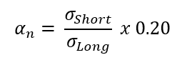
Therefore, the alpha is calculated as a ratio between a short-term volatility calculation and a long-term volatility calculation. The result is multiplied by 0.20. Then, to calculate the VAMA, we follow these steps.

The first VAMA value is simply the closing price, and then the algorithm can take the form of the above formula.

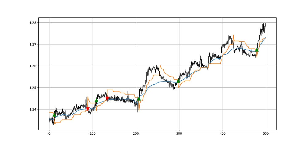
The above chart shows the USDCAD hourly values with the VAMA using a 3-period standard deviation and a 55-period standard deviation. To code the VAMA, we use the below function
def volatility_adjusted_moving_average(Data, lookback_volatility_short, lookback_volatility_long, close, where):

    # Adding Columns
    Data = adder(Data, 2)

    # Calculating Standard Deviations
    Data = volatility(Data, lookback_volatility_short, close, where)
    Data = volatility(Data, lookback_volatility_long, close, where + 1)

    # Calculating Alpha
    for i in range(len(Data)):

        Data[i, where + 2] = 0.2 * (Data[i, where] / Data[i, where + 1])

    # Calculating the First Value of VAMA
    Data[1, where + 3] = (Data[1, where + 2] * Data[1, close]) + ((1 - Data[1, where + 2]) * Data[0, close])

    # Calculating the Rest of VAMA
    for i in range(2, len(Data)):

        Data[i, where + 3] = (Data[i, where + 2] * Data[i, close]) + ((1 - Data[i, where + 2]) * Data[i - 1, where + 3])

    # Cleaning
    Data = deleter(Data, where, 3)
    Data = jump(Data, 1)

    return Data
The way to use the VAMA is to follow the trend with it or simply expect reactions from it whenever the market approaches it. There are a lot of combinations to be made with this moving average, so be creative!
The SuperTrend Indicator
The first concept we should understand before creating the SuperTrend indicator is volatility. We sometimes measure volatility using the Average True Range. Although the ATR is considered a lagging indicator, it gives some insights as to where volatility is right now and where has it been last period (day, week, month, etc.). But before that, we should understand how the True Range is calculated (the ATR is just the average of that calculation).
The true range is simply the greatest of the three price differences:
High — Low
| High — Previous close |
| Previous close — Low |
Once we have gotten the maximum out of the above three, we simply take an average of n periods of the true ranges to get the Average True Range. Generally, since in periods of panic and price depreciation we see volatility go up, the ATR will most likely trend higher during these periods, similarly in times of steady uptrends or downtrends, the ATR will tend to go lower.
One should always remember that this indicator is lagging and therefore has to be used with extreme caution. Below is the function code that calculates the ATR. Make sure you have an OHLC array of historical data.
def atr(data, lookback, high, low, close, where):

    # adding columns
    data = adder(data, 2)

    # true range
    for i in range(len(data)):

        try:

            data[i, where] = max(data[i, high] - data[i, low], abs(data[i, high] - data[i - 1, close]), abs(data[i, low]  - data[i - 1, close]))

        except ValueError:

            pass

    data[0, where] = 0

    # average true range
    data = ema(data, 2, (lookback * 2) - 1, where, where + 1)

    # Cleaning
    data = deleter(data, where, 1)
    data = jump(data, lookback)

    return data
Now that we have understood what the ATR is and how to calculate it, we can proceed further with the SuperTrend indicator. The indicator seeks to provide entry and exit levels for trend followers. You can think of it as a moving average or an MACD. Its uniqueness is its main advantage and although its calculation method is much more complicated than the other two indicators, it is intuitive in nature and not that hard to understand. Basically, we have two variables to choose from.
The ATR lookback and the multiplier’s value. The former is just the period used to calculated the ATR while the latter is generally an integer (usually 2 or 3).

The first thing to do is to average the high and low of the price bar, then we will either add or subtract the average with the selected multiplier multiplied by the ATR as shown in the above formulas. This will give us two arrays, the basic upper band and the basic lower band which form the first building blocks in the SuperTrend indicator. The next step is to calculate the final upper band and the final lower band using the below formulas.


It may seem complicated but most of these conditions are repetitive and in any case, I will provide the Python code below so that you can play with the function and optimize it to your trading preferences. Finally, using the previous two calculations, we can find the SuperTrend.

def supertrend(Data, multiplier, atr_col, close, high, low, where):

    Data = adder(Data, 6)

    for i in range(len(Data)):

            # Average Price
            Data[i, where] = (Data[i, high] + Data[i, low]) / 2
            # Basic Upper Band
            Data[i, where + 1] = Data[i, where] + (multiplier * Data[i, atr_col])
            # Lower Upper Band
            Data[i, where + 2] = Data[i, where] - (multiplier * Data[i, atr_col])

    # Final Upper Band
    for i in range(len(Data)):

        if i == 0:
            Data[i, where + 3] = 0

        else:
            if (Data[i, where + 1] < Data[i - 1, where + 3]) or (Data[i - 1, close] > Data[i - 1, where + 3]):
                Data[i, where + 3] = Data[i, where + 1]

            else:
                Data[i, where + 3] = Data[i - 1, where + 3]

    # Final Lower Band
    for i in range(len(Data)):

        if i == 0:
            Data[i, where + 4] = 0

        else:
            if (Data[i, where + 2] > Data[i - 1, where + 4]) or (Data[i - 1, close] < Data[i - 1, where + 4]):
                Data[i, where + 4] = Data[i, where + 2]

            else:
                Data[i, where + 4] = Data[i - 1, where + 4]

    # SuperTrend
    for i in range(len(Data)):

        if i == 0:
            Data[i, where + 5] = 0

        elif (Data[i - 1, where + 5] == Data[i - 1, where + 3]) and (Data[i, close] <= Data[i, where + 3]):
            Data[i, where + 5] = Data[i, where + 3]

        elif (Data[i - 1, where + 5] == Data[i - 1, where + 3]) and (Data[i, close] >  Data[i, where + 3]):
            Data[i, where + 5] = Data[i, where + 4]

        elif (Data[i - 1, where + 5] == Data[i - 1, where + 4]) and (Data[i, close] >= Data[i, where + 4]):
            Data[i, where + 5] = Data[i, where + 4]

        elif (Data[i - 1, where + 5] == Data[i - 1, where + 4]) and (Data[i, close] <  Data[i, where + 4]):
            Data[i, where + 5] = Data[i, where + 3]

    # Cleaning columns
    Data = deleter(Data, where, 5)

    return Data
The above chart shows the hourly values of the EURUSD with a 10-period SuperTrend (represented by the ATR period) and a multiplier of 3. The way we should understand the indicator is that when it goes above the market price, we should be looking to short and when it goes below the market price, we should be looking to go long as we anticipate a bullish trend. Remember that the SuperTrend is a trend-following indicator. The aim here is to capture trends at the beginning and to close out when they are over.
If you are also interested by more technical indicators and strategies, then my book might interest you:
Creating the Strategy
The strategy relies on the double confirmation from both indicators. We generally use the SuperTrend for the trigger and the volatility-adjusted moving average for confirmation. The below are the conditions:
A long (Buy) signal is generated whenever the market surpasses the SuperTrend(10, 3) while being above the volatility-adjusted moving average(3, 55).
A short (Sell) signal is generated whenever the market breaks the SuperTrend(10, 3) while being below the volatility-adjusted moving average(3, 55).
def signal(data, close, vama_column, super_trend_column, buy_column, sell_column):

    data = adder(data, 10)

    for i in range(len(data)):

        if data[i, close] > data[i, super_trend_column] and data[i, close] > data[i, vama_column] and data[i - 1, close] < data[i - 1, super_trend_column]:

            data[i, buy_column] = 1

        if data[i, close] < data[i, super_trend_column] and data[i, close] < data[i, vama_column] and data[i - 1, close] > data[i - 1, super_trend_column]:

            data[i, sell_column] = -1

    return data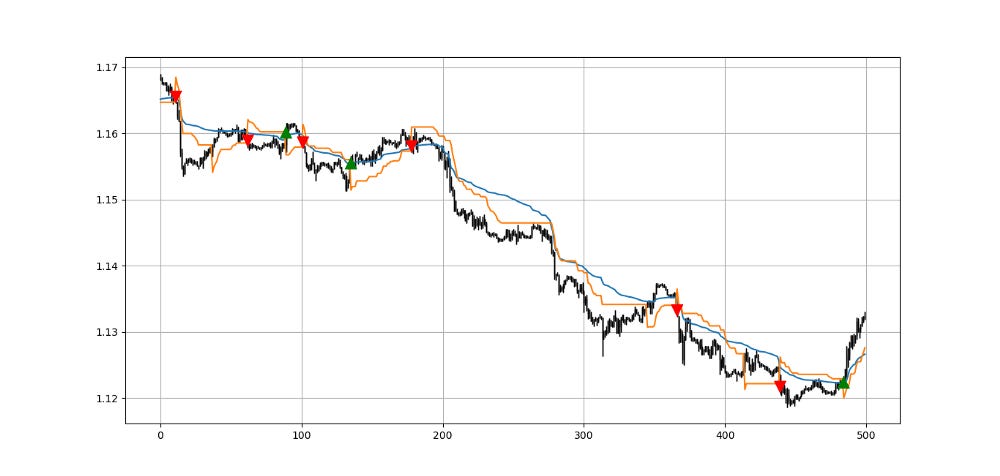
Conclusion
Remember to always do your back-tests. You should always believe that other people are wrong. My indicators and style of trading may work for me but maybe not for you.
I am a firm believer of not spoon-feeding. I have learnt by doing and not by copying. You should get the idea, the function, the intuition, the conditions of the strategy, and then elaborate (an even better) one yourself so that you back-test and improve it before deciding to take it live or to eliminate it. My choice of not providing specific Back-testing results should lead the reader to explore more herself the strategy and work on it more.
To sum up, are the strategies I provide realistic? Yes, but only by optimizing the environment (robust algorithm, low costs, honest broker, proper risk management, and order management). Are the strategies provided only for the sole use of trading? No, it is to stimulate brainstorming and getting more trading ideas as we are all sick of hearing about an oversold RSI as a reason to go short or a resistance being surpassed as a reason to go long. I am trying to introduce a new field called Objective Technical Analysis where we use hard data to judge our techniques rather than rely on outdated classical methods.