


Combining the SuperTrend With the RSI
How to Create a Trend-Following Strategy in Python


Trend following strategies rely on confirmation techniques to detect as early as possible a new trend. This article discusses a strategy on the RSI and the SuperTrend.
The Relative Strength Index
First introduced by J. Welles Wilder Jr., the RSI is one of the most popular and versatile technical indicators. Mainly used as a contrarian indicator where extreme values signal a reaction that can be exploited. Typically, we use the following steps to calculate the default RSI:
Calculate the change in the closing prices from the previous ones.
Separate the positive net changes from the negative net changes.
Calculate a smoothed moving average on the positive net changes and on the absolute values of the negative net changes.
Divide the smoothed positive changes by the smoothed negative changes. We will refer to this calculation as the Relative Strength — RS.
Apply the normalization formula shown below for every time step to get the RSI.
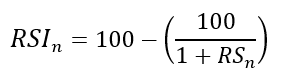

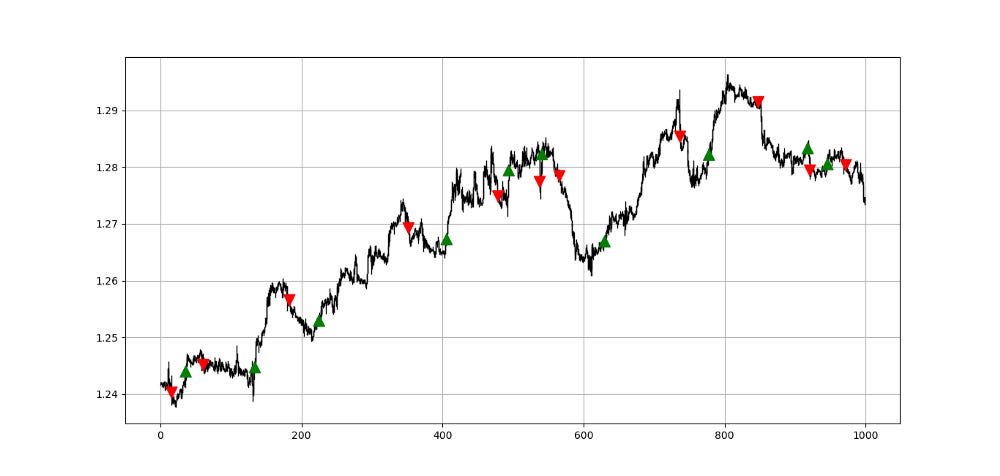
The above chart shows the hourly values of the GBPUSD in black with the 13-period RSI. We can generally note that the RSI tends to bounce close to 25 while it tends to pause around 75. To code the RSI in Python, we need an OHLC array composed of four columns that cover open, high, low, and close prices.
def add_column(data, times):

    for i in range(1, times + 1):

        new = np.zeros((len(data), 1), dtype = float)

        data = np.append(data, new, axis = 1)
return datadef delete_column(data, index, times):
for i in range(1, times + 1):
data = np.delete(data, index, axis = 1)return datadef delete_row(data, number):
data = data[number:, ]
return datadef ma(data, lookback, close, position):
data = add_column(data, 1)
for i in range(len(data)):
try:
data[i, position] = (data[i - lookback + 1:i + 1, close].mean())
except IndexError:
pass
data = delete_row(data, lookback)
return datadef smoothed_ma(data, alpha, lookback, close, position):
lookback = (2 * lookback) - 1
alpha = alpha / (lookback + 1.0)
beta = 1 - alpha
data = ma(data, lookback, close, position)data[lookback + 1, position] = (data[lookback + 1, close] * alpha) + (data[lookback, position] * beta)for i in range(lookback + 2, len(data)):
try:
data[i, position] = (data[i, close] * alpha) + (data[i - 1, position] * beta)
except IndexError:
pass
return datadef rsi(data, lookback, close, position):
data = add_column(data, 5)
for i in range(len(data)):
data[i, position] = data[i, close] - data[i - 1, close]
for i in range(len(data)):
if data[i, position] > 0:
data[i, position + 1] = data[i, position]
elif data[i, position] < 0:
data[i, position + 2] = abs(data[i, position])
data = smoothed_ma(data, 2, lookback, position + 1, position + 3)
data = smoothed_ma(data, 2, lookback, position + 2, position + 4)data[:, position + 5] = data[:, position + 3] / data[:, position + 4]
data[:, position + 6] = (100 - (100 / (1 + data[:, position + 5])))data = delete_column(data, position, 6)
data = delete_row(data, lookback)return dataMake sure to focus on the concepts and not the code. You can find the codes of most of my strategies in my books. The most important thing is to comprehend the techniques and strategies.
Knowledge must be accessible to everyone. This is why, from now on, a purchase of either one of my new books “Contrarian Trading Strategies in Python” or “Trend Following Strategies in Python” comes with free PDF copies of my first three books (Therefore, purchasing one of the new books gets you 4 books in total). The two new books listed above feature a lot of advanced indicators and strategies with a GitHub page. You can use the below link to purchase one of the two books (Please specify which one and make sure to include your e-mail in the note).
Pay Kaabar using PayPal.Me
Go to paypal.me/sofienkaabar and type in the amount. Since it’s PayPal, it’s easy and secure. Don’t have a PayPal…www.paypal.com
The SuperTrend
The first concept we should understand before creating the SuperTrend indicator is volatility. We sometimes measure volatility using the average true range. Although the ATR is considered a lagging indicator, it gives some insights as to where volatility is right now and where has it been last period (day, week, month, etc.). But before that, we should understand how the true range is calculated (the ATR is just the average of that calculation). The true range is simply the greatest of the three price differences:
High — Low
| High — Previous close |
| Previous close — Low |
Once we have gotten the maximum out of the above three, we simply take an average of n periods of the true ranges to get the average true range. Generally, since in periods of panic and price depreciation we see volatility go up, the ATR will most likely trend higher during these periods, similarly in times of steady uptrends or downtrends, the ATR will tend to go lower.
One should always remember that this indicator is lagging and therefore has to be used with extreme caution. Below is the function code that calculates the ATR. Make sure you have an OHLC array of historical data.
def atr(data, lookback, high, low, close, where):

    data = adder(data, 1)

    for i in range(len(data)):

        try:

            data[i, where] = max(data[i, high] - data[i, low], abs(data[i, high] - data[i - 1, close]), abs(data[i, low]  - data[i - 1, close]))

        except ValueError:

            pass

    data[0, where] = 0

    data = ema(data, 2, (lookback * 2) - 1, where, where + 1)
data = deleter(data, where, 1)
data = jump(data, lookback)
return dataNow that we have understood what the ATR is and how to calculate it, we can proceed further with the SuperTrend indicator. The indicator seeks to provide entry and exit levels for trend followers. You can think of it as a moving average or an MACD. Its uniqueness is its main advantage and although its calculation method is much more complicated than the other two indicators, it is intuitive in nature and not that hard to understand. Basically, we have two variables to choose from. The ATR lookback and the multiplier’s value. The former is just the period used to calculated the ATR while the latter is generally an integer (usually 2 or 3).

The first thing to do is to average the high and low of the price bar, then we will either add or subtract the average with the selected multiplier multiplied by the ATR as shown in the above formulas. This will give us two arrays, the basic upper band and the basic lower band which form the first building blocks in the SuperTrend indicator. The next step is to calculate the final upper band and the final lower band using the below formulas.


It may seem complicated but most of these conditions are repetitive and in any case, I will provide the Python code below so that you can play with the function and optimize it to your trading preferences. Finally, using the previous two calculations, we can find the SuperTrend.

def supertrend(data, multiplier, high, low, close, atr_col, where):

    data = adder(data, 6)

    for i in range(len(data)):

            data[i, where] = (data[i, high] + data[i, low]) / 2

            data[i, where + 1] = data[i, where] + (multiplier * data[i, atr_col])

            data[i, where + 2] = data[i, where] - (multiplier * data[i, atr_col])

    for i in range(len(data)):

        if i == 0:

            data[i, where + 3] = 0

        else:

            if (data[i, where + 1] < data[i - 1, where + 3]) or (data[i - 1, close] > data[i - 1, where + 3]):

                data[i, where + 3] = data[i, where + 1]

            else:

                data[i, where + 3] = data[i - 1, where + 3]

    for i in range(len(data)):

        if i == 0:

            data[i, where + 4] = 0

        else:

            if (data[i, where + 2] > data[i - 1, where + 4]) or (data[i - 1, close] < data[i - 1, where + 4]):

                data[i, where + 4] = data[i, where + 2]

            else:

                data[i, where + 4] = data[i - 1, where + 4]

    for i in range(len(data)):

        if i == 0:

            data[i, where + 5] = 0

        elif (data[i - 1, where + 5] == data[i - 1, where + 3]) and (data[i, close] <= data[i, where + 3]):

            data[i, where + 5] = data[i, where + 3]

        elif (data[i - 1, where + 5] == data[i - 1, where + 3]) and (data[i, close] >  data[i, where + 3]):

            data[i, where + 5] = data[i, where + 4]

        elif (data[i - 1, where + 5] == data[i - 1, where + 4]) and (data[i, close] >= data[i, where + 4]):

            data[i, where + 5] = data[i, where + 4]

        elif (data[i - 1, where + 5] == data[i - 1, where + 4]) and (data[i, close] <  data[i, where + 4]):

            data[i, where + 5] = data[i, where + 3]

    data = deleter(data, where, 5)
data = jump(data, 1)
return data
The above chart shows the hourly values of the EURUSD with a 10-period SuperTrend (represented by the ATR period) and a multiplier of 3. The way we should understand the indicator is that when it goes above the market price, we should be looking to short and when it goes below the market price, we should be looking to go long as we anticipate a bullish trend. Remember that the SuperTrend is a trend-following indicator. The aim here is to capture trends at the beginning and to close out when they are over.
Creating the Strategy
The strategy relies on signals from the SuperTrend and confirmation from the RSI. Here are the trading conditions keeping in mind that the parameters and the lookbacks must be tweaked in order to minimize lag and optimize the triggers:
Long (Buy) whenever the market surpasses the SuperTrend while the RSI is above 50.
Short (Sell) whenever the market breaks the SuperTrend while the RSI is below 50.
def signal(data, close, rsi_column, supertrend_column, buy, sell):
    data = adder(data, 5)
    for i in range(len(data)):

        if data[i, rsi_column] > 50 and data[i, close] > data[i, supertrend_column] and data[i - 1, close] < data[i - 1, supertrend_column]:

            data[i, buy] = 1

        if data[i, rsi_column] < 50 and data[i, close] < data[i, supertrend_column] and data[i - 1, close] > data[i - 1, supertrend_column]:

            data[i, sell] = -1

    return data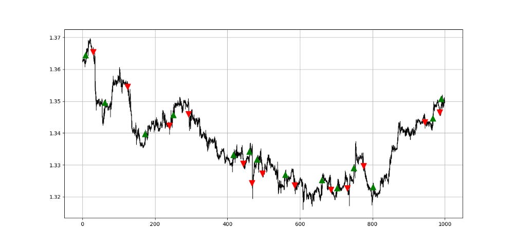
If you want to see how to create all sorts of algorithms yourself, feel free to check out Lumiwealth. From algorithmic trading to blockchain and machine learning, they have hands-on detailed courses that I highly recommend.
Learn Algorithmic Trading with Python Lumiwealth
Learn how to create your own trading algorithms for stocks, options, crypto and more from the experts at Lumiwealth. Click to learn more
Summary
To sum up, what I am trying to do is to simply contribute to the world of objective technical analysis which is promoting more transparent techniques and strategies that need to be back-tested before being implemented. This way, technical analysis will get rid of the bad reputation of being subjective and scientifically unfounded.
I recommend you always follow the the below steps whenever you come across a trading technique or strategy:
Have a critical mindset and get rid of any emotions.
Back-test it using real life simulation and conditions.
If you find potential, try optimizing it and running a forward test.
Always include transaction costs and any slippage simulation in your tests.
Always include risk management and position sizing in your tests.
Finally, even after making sure of the above, stay careful and monitor the strategy because market dynamics may shift and make the strategy unprofitable.