Combining the Simple RSI & the Stochastic Oscillator in a Trading Strategy
Creating a Combined Strategy Using & the Simple RSI & the Stochastic Oscillator
Combining strategies is always the right path towards a robust system. But does combining simple default indicators result in positive results? In this article, the simple RSI seen in a previous article and the stochastic oscillator are used together to provide signals, the idea is to code them and see the results.
Medium is a hub to interesting reads. I read a lot of articles before I decided to start writing. Consider joining Medium using my referral link (at NO additional cost to you).
Join Medium with my referral link — Sofien Kaabar
As a Medium member, a portion of your membership fee goes to writers you read, and you get full access to every story…kaabar-sofien.medium.com
The Relative Strength Index
First introduced by J. Welles Wilder Jr., the RSI is one of the most popular and versatile technical indicators. Mainly used as a contrarian indicator where extreme values signal a reaction that can be exploited. Typically, we use the following steps to calculate the default RSI:
Calculate the change in the closing prices from the previous ones.
Separate the positive net changes from the negative net changes.
Calculate a smoothed moving average on the positive net changes and on the absolute values of the negative net changes.
Divide the smoothed positive changes by the smoothed negative changes. We will refer to this calculation as the Relative Strength — RS.
Apply the normalization formula shown below for every time step to get the RSI.
The above chart shows the hourly values of the GBPUSD in black with the 13-period RSI. We can generally note that the RSI tends to bounce close to 25 while it tends to pause around 75. To code the RSI in Python, we need an OHLC array composed of four columns that cover open, high, low, and close prices.
def adder(data, times):

    for i in range(1, times + 1):

        new = np.zeros((len(data), 1), dtype = float)

        data = np.append(data, new, axis = 1)
return datadef deleter(data, index, times):
for i in range(1, times + 1):
data = np.delete(data, index, axis = 1)return data
def jump(data, jump):
data = data[jump:, ]
return datadef ma(data, lookback, close, where):
data = adder(data, 1)
for i in range(len(data)):
try:
data[i, where] = (data[i - lookback + 1:i + 1, close].mean())
except IndexError:
pass
data = jump(data, lookback)
return datadef ema(data, alpha, lookback, what, where):
alpha = alpha / (lookback + 1.0)
beta = 1 - alpha
data = ma(data, lookback, what, where)data[lookback + 1, where] = (data[lookback + 1, what] * alpha) + (data[lookback, where] * beta)for i in range(lookback + 2, len(data)):
try:
data[i, where] = (data[i, what] * alpha) + (data[i - 1, where] * beta)
except IndexError:
pass
return datadef rsi(data, lookback, close, where):
data = adder(data, 5)
for i in range(len(data)):
data[i, where] = data[i, close] - data[i - 1, close]
for i in range(len(data)):
if data[i, where] > 0:
data[i, where + 1] = data[i, where]
elif data[i, where] < 0:
data[i, where + 2] = abs(data[i, where])
lookback = (lookback * 2) - 1 # From exponential to smoothed
data = ema(data, 2, lookback, where + 1, where + 3)
data = ema(data, 2, lookback, where + 2, where + 4)data[:, where + 5] = data[:, where + 3] / data[:, where + 4]
data[:, where + 6] = (100 - (100 / (1 + data[:, where + 5])))data = deleter(data, where, 6)
data = jump(data, lookback)return dataKnowledge must be accessible to everyone. This is why, from now on, a purchase of either one of my new books “Contrarian Trading Strategies in Python” or “Trend Following Strategies in Python” comes with free PDF copies of my first three books (Therefore, purchasing one of the new books gets you 4 books in total). The two new books listed above feature a lot of advanced indicators and strategies with a GitHub page. You can use the below link to purchase one of the two books (Please specify which one and make sure to include your e-mail in the note).
Pay Kaabar using PayPal.Me
Go to paypal.me/sofienkaabar and type in the amount. Since it’s PayPal, it’s easy and secure. Don’t have a PayPal…www.paypal.com
The Simple Relative Strength Index
The simple RSI is a simple change in the way the moving average is calculated inside the formula of the standard RSI. Instead of using a smoothed moving average as recommended by Wilder, we will use a simple moving average. Therefore, in the function provided above, we already have the choice and hence, we can write directly the following code:
my_data = rsi(my_data, 14, 3, 4, genre = 'Simple')# The 14 refers to the lookback period on the RSI
# The 3 refers to the closing prices on the OHLC array
# The 4 refers to the index of the column where the RSI will be putThe Stochastic Oscillator
This great technique allows us to trap the values between 0 and 1 (or 0 and 100 if we wish to multiply by 100). The concept revolves around subtracting the minimum value in a certain lookback period from the current value and dividing by the maximum value in the same lookback period minus the minimum value (the same in the nominator).
We can try to code the function of normalization in python. The below normalizes a given time series:
def normalizer(Data, lookback, what, where):

    for i in range(len(Data)):

        try:
            Data[i, where] = (Data[i, what] - min(Data[i - lookback + 1:i + 1, what])) / (max(Data[i - lookback + 1:i + 1, what]) - min(Data[i - lookback + 1:i + 1, what]))

        except ValueError:
            pass

    Data[:, where] = Data[:, where] * 100
    Data = jump(Data, lookback)
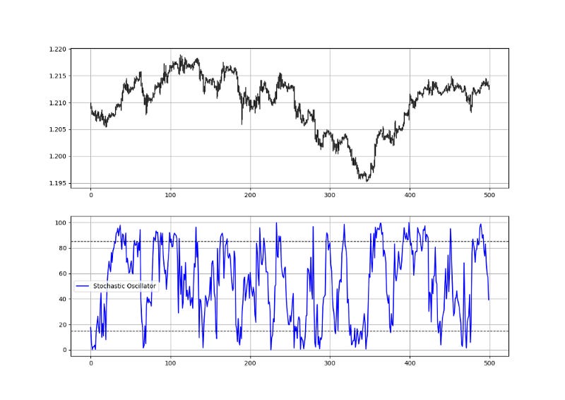
return DataIf we apply the function to the closing price of the EURUSD hourly time frame with a 50 lookback period (meaning, the function will look at the last 50 values and select the minimum and maximum values from there) we will have the following chart.
# Using the function
my_data = normalizer(my_data, 50, 3, 4)
The stochastic oscillator seeks to find oversold and overbought zones by incorporating the highs and lows using the normalization formula as shown below:
An overbought level is an area where the market is perceived to be extremely bullish and is bound to consolidate. An oversold level is an area where market is perceived to be extremely bearish and is bound to bounce. Hence, the Stochastic Oscillator is a contrarian indicator that seeks to signal reactions of extreme movements.
We will create the below function that calculates the Stochastic on an OHLC data:
def stochastic(Data, lookback, what, high, low, where):

    for i in range(len(Data)):

        try:
          Data[i, where] = (Data[i, what] - min(Data[i - lookback + 1:i + 1, low])) / (max(Data[i - lookback + 1:i + 1, high]) - min(Data[i - lookback + 1:i + 1, low]))

        except ValueError:
            pass

    Data[:, where] = Data[:, where] * 100
return Data# The Data variable refers to the OHLC array
# The lookback variable refers to the period (5, 14, 21, etc.)
# The what variable refers to the closing price
# The high variable refers to the high price
# The low variable refers to the low price
# The where variable refers to where to put the OscillatorThe above plot shows the EURUSD values plotted with a 14-period stochastic oscillator. Notice that the indicator will always be bounded between 0 and 100 due to the nature of its normalization function that traps values between the minimum and the maximum.
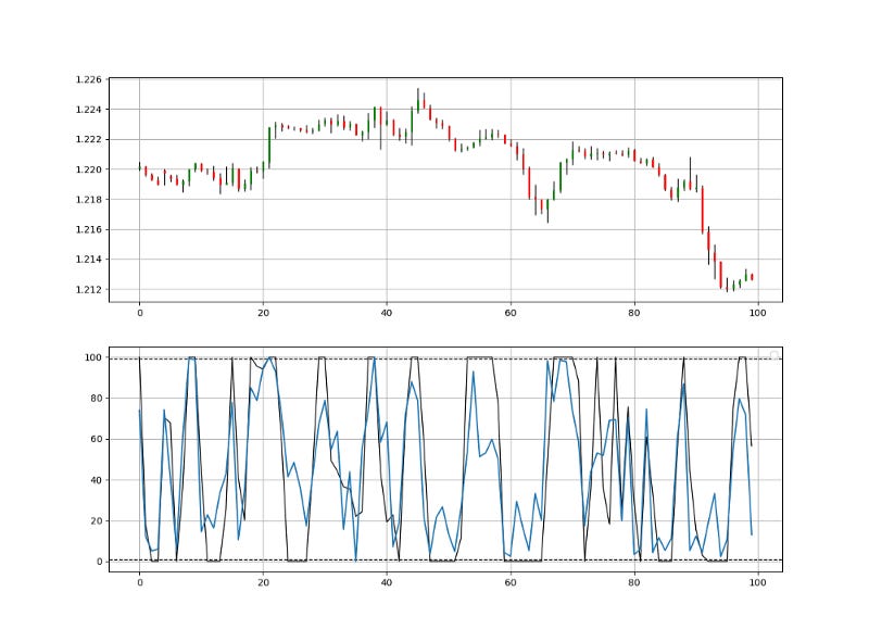
As with any proper research method, the aim is to be able to see for ourselves whether it is worth having as an add-on to our pre-existing trading framework. The below plot shows the hourly EURUSD values in the first panel with the two indicators plotted in the second panel. The following are the parameters:
2-period Simple Relative Strength Index.
2-period Stochastic Oscillator.
99 as the upper barrier and 1 as the lower barrier.
We put 1 and 99 as 0 and 100 are not really possible due to the formula of the stochastic oscillator. The below signal chart shows the triggers we have gotten from following the below conditions.
The conditions of the strategy are as follows:
Long (Buy) whenever the 2-period simple RSI and the 2-period stochastic oscillator are below 1 simultaneously.
Short (Sell) whenever the 2-period simple RSI and the 2-period stochastic oscillator are above 99 simultaneously.
upper_barrier    = 99
lower_barrier    = 1
def signal(Data, rsi_col, stoch_col, buy, sell):
Data = adder(Data, 10)
Data = rounding(Data, 5)
for i in range(len(Data)):
if Data[i, rsi_col] < lower_barrier and Data[i, stoch_col] < lower_barrier:
Data[i, buy] = 1
elif Data[i, rsi_col] > upper_barrier and Data[i, stoch_col] > upper_barrier:
Data[i, sell] = -1
return DataRemember to always do your back-tests. You should always believe that other people are wrong. My indicators and style of trading may work for me but maybe not for you.
I am a firm believer of not spoon-feeding. I have learnt by doing and not by copying. You should get the idea, the function, the intuition, the conditions of the strategy, and then elaborate (an even better) one yourself so that you back-test and improve it before deciding to take it live or to eliminate it. My choice of not providing specific Back-testing results should lead the reader to explore more herself the strategy and work on it more.
If you want to see how to create all sorts of algorithms yourself, feel free to check out Lumiwealth. From algorithmic trading to blockchain and machine learning, they have hands-on detailed courses that I highly recommend.
Learn Algorithmic Trading with Python Lumiwealth
Learn how to create your own trading algorithms for stocks, options, crypto and more from the experts at Lumiwealth. Click to learn more
Summary
To sum up, what I am trying to do is to simply contribute to the world of objective technical analysis which is promoting more transparent techniques and strategies that need to be back-tested before being implemented. This way, technical analysis will get rid of the bad reputation of being subjective and scientifically unfounded.
I recommend you always follow the the below steps whenever you come across a trading technique or strategy:
Have a critical mindset and get rid of any emotions.
Back-test it using real life simulation and conditions.
If you find potential, try optimizing it and running a forward test.
Always include transaction costs and any slippage simulation in your tests.
Always include risk management and position sizing in your tests.
Finally, even after making sure of the above, stay careful and monitor the strategy because market dynamics may shift and make the strategy unprofitable.


