Buying the Dips & Selling the Strength Trading Strategy in Python.
Creating & Evaluating the Dips Trading Strategy Using Python.
One of the first things we are taught in trading 101 are moving averages. Their simplicity and efficiency as well as their scientific robustness is enough to make them one of the most appealing technical indicators. They belong to the overlay family as they are charted along the market price and not separately like the RSI. We are often taught to use their crossovers as trading signals that imply a change of direction and a beginning of a new trend. However, there are many ways of using them as well, one of these ways is the dip strategy or what I like to refer to as the dynamic reaction strategy.
I have just published a new book after the success of my previous one “New Technical Indicatorsin Python”. It features a more complete description and addition of structured trading strategies with a Github page dedicated to the continuously updated code. If you feel that this interests you, feel free to visit the below link, or if you prefer to buy the PDF version, you could contact me on Linkedin.
The Book of Trading Strategies
Amazon.com: The Book of Trading Strategies: 9798532885707: Kaabar, Sofien: Bookswww.amazon.com
Moving Averages: An Introduction
Moving averages help us confirm and ride the trend. They are the most known technical indicator and this is because of their simplicity and their proven track record of adding value to the analyses. We can use them to find support and resistance levels, stops and targets, and to understand the underlying trend. This versatility makes them an indispensable tool in our trading arsenal.
As the name suggests, this is your plain simple mean that is used everywhere in statistics and basically any other part in our lives. It is simply the total values of the observations divided by the number of observations. Mathematically speaking, it can be written down as:
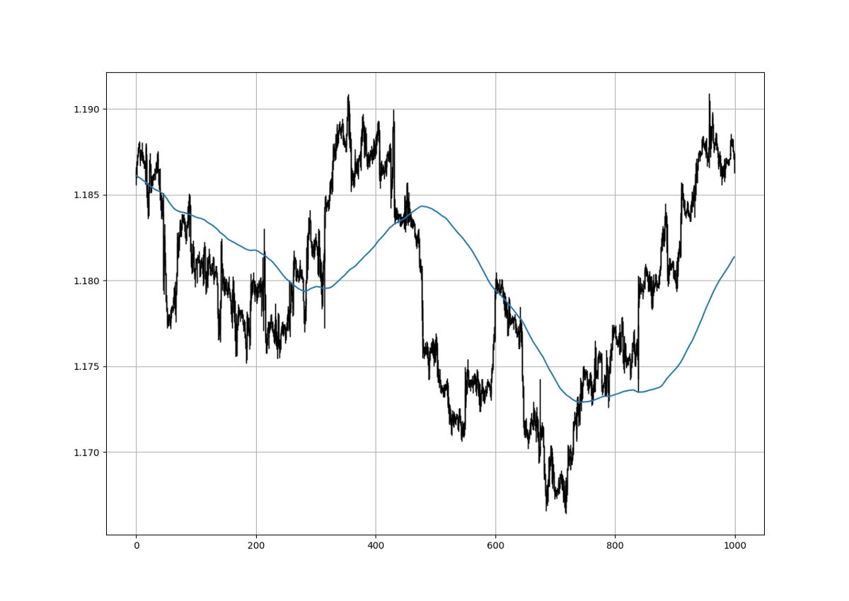
We can see that the moving average is providing decent dynamic support and resistance levels from where we can place our orders in case the market goes down there. The code for the moving average can be written down as the following:
def adder(Data, times):

    for i in range(1, times + 1):

        new = np.zeros((len(Data), 1), dtype = float)
        Data = np.append(Data, new, axis = 1)

    return Data

def deleter(Data, index, times):

    for i in range(1, times + 1):

        Data = np.delete(Data, index, axis = 1)

    return Data

def jump(Data, jump):

    Data = Data[jump:, ]

    return Data

def ma(Data, lookback, close, where):

    Data = adder(Data, 1)

    for i in range(len(Data)):

            try:
                Data[i, where] = (Data[i - lookback + 1:i + 1, close].mean())

            except IndexError:
                pass

    # Cleaning
    Data = jump(Data, lookback)

    return Data
The below states that the moving average function will be called on the array named my_data for a lookback period of 233, on the column indexed at 3 (closing prices in an OHLC array). The moving average values will then be put in the column indexed at 4 which is the one we have added using the adder function.
my_data = ma(my_data, 233, 3, 4)The choice of 233 is purely subjective as many traders use 200 or 250 while some (like me) prefer 233.
The Dips Trading Strategy
Moving averages are a great way of finding objective support and resistance levels and this makes it easier for us to determine where we can buy the dips to follow a move upwards and where we can sell the strengths to follow a move downwards in case short-selling is allowed. The trading rules are:
A long (Buy) signal is generated whenever the market price approaches its moving average from the above. This is because we are anticipating a bullish reaction within the bullish trend.
A short (Sell) signal is generated whenever the market price approaches its moving average from the below. This is because we are anticipating a bearish reaction within the bearish trend.
lookback = 233
distance = 0.0003The syntax for the above conditions can be shown in the below code snippet.
def signal(Data, high, low, close, ma_col, buy, sell):

    Data = adder(Data, 10)

    for i in range(len(Data)):

        if Data[i, low] > Data[i, ma_col] and abs(Data[i, low] - Data[i, ma_col]) < distance and \
           Data[i - 1, buy] == 0 and Data[i - 2, buy] == 0 and Data[i - 3, buy] == 0 and \
           Data[i - 1, sell] == 0 and Data[i - 2, sell] == 0 and Data[i - 3, sell] == 0 and \
           Data[i - 13, close] > Data[i - 13, ma_col] and Data[i - 1, close] > Data[i, close]:

            Data[i, buy] = 1

        elif Data[i, high] < Data[i, ma_col] and abs(Data[i, ma_col] - Data[i, high]) < distance and \
             Data[i - 1, buy] == 0 and Data[i - 2, buy] == 0 and Data[i - 3, buy] == 0 and \
             Data[i - 1, sell] == 0 and Data[i - 2, sell] == 0 and Data[i - 3, sell] == 0 and \
           Data[i - 13, close] < Data[i - 13, ma_col] and Data[i - 1, close] < Data[i, close]:

            Data[i, sell] = -1

    return Data

# Adding a few columns to the OHLC array
my_data = adder(my_data, 10)

# Calling the moving average function
my_data = ma(my_data, lookback, 3, 4)

# Calling the signal function
my_data = signal(my_data, 1, 2, 3, 4, 6, 7)
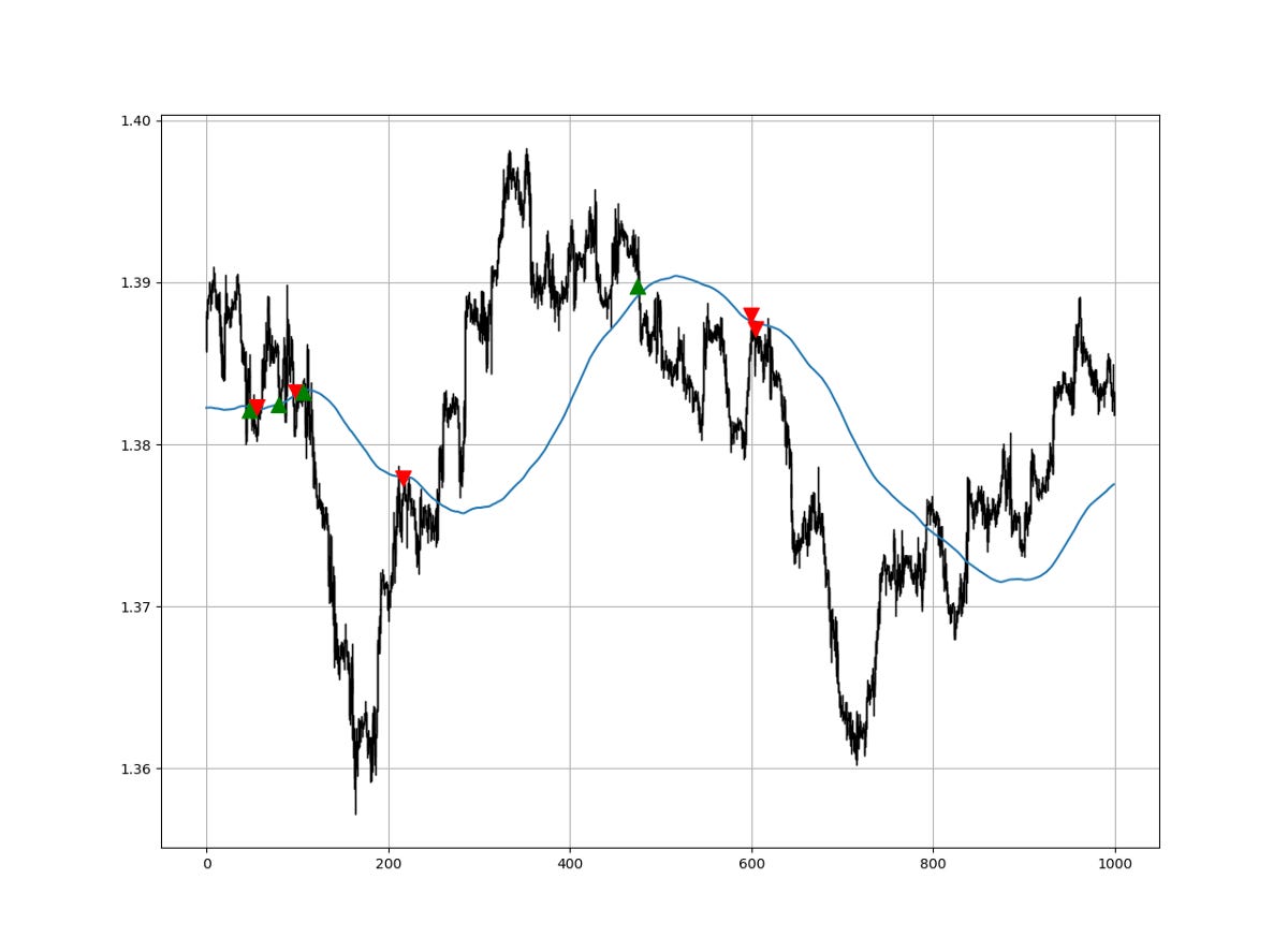
We need to tell the signal function that is must loop chronologically around the historical OHLC data, find the minimum distance between the market price and its moving average while respecting certain conditions, and then input 1 in the buy column or -1 in the sell column. This way we will be able to visualize and count the number of signals on the selected charts.
The above chart shows a sample of the generated signals based on the conditions we have imposed. We can notice that there are more conditions in the signal function. This is so that the algorithm does not include certain exceptional events as trading signals. We need to filter it as much as we can and even the signal function we have written does not cover everything. For example, we have included the condition that the previous closing price must be higher than the current closing price in case of a bullish configuration. Also, to avoid breakouts and re-integrations, we have included a subjective condition stating that for a bullish configuration, the closing price 13 periods ago must be greather than the moving average 13 periods ago. We can tweak the signal function as much as we can.
Now, what if we make the moving average more long-term so that we profit from a wider window? Remember we have discussed a certain moving average that I like to use all the time, that is the 800-period moving average.
lookback = 800
distance = 0.0003The distance variable is the minimum distance between the low/high price and the moving average so that the algorithm considers it to be an opportunity. In other words, for a bearish configuration, if the current high is less than 3 pips away from the current moving average and is below it, then a bearish signal is triggered if the other conditions are also satisfied.
The 800-period moving average may offer more stability and less frequent signals. Let us know evaluate the signals using one simple neutral prediction metric, the signal quality.
If you are also interested by more technical indicators and using Python to create strategies, then my best-selling book on Technical Indicators may interest you:
New Technical Indicators in Python
Amazon.com: New Technical Indicators in Python: 9798711128861: Kaabar, Mr Sofien: Bookswww.amazon.com
Evaluating the Strategy
Having had the signals, we now know when the algorithm would have placed its buy and sell orders, meaning, that we have an approximate replica of the past where can can control our decisions with no hindsight bias. We have to simulate how the strategy would have done given our conditions. This means that we need to calculate the returns and analyze the performance metrics. Let us see a neutral metric that can give us somewhat a clue on the predictability of the indicator or the strategy. For this study, we will use the Signal Quality metric.
The signal quality is a metric that resembles a fixed holding period strategy. It is simply the reaction of the market after a specified time period following the signal. Generally, when trading, we tend to use a variable period where we open the positions and close out when we get a signal on the other direction or when we get stopped out (either positively or negatively).
Sometimes, we close out at random time periods. Therefore, the signal quality is a very simple measure that assumes a fixed holding period and then checks the market level at that time point to compare it with the entry level. In other words, it measures market timing by checking the reaction of the market after a specified time period.
Conclusion
Remember to always do your back-tests. You should always believe that other people are wrong. My indicators and style of trading may work for me but maybe not for you.
I am a firm believer of not spoon-feeding. I have learnt by doing and not by copying. You should get the idea, the function, the intuition, the conditions of the strategy, and then elaborate (an even better) one yourself so that you back-test and improve it before deciding to take it live or to eliminate it. My choice of not providing specific Back-testing results should lead the reader to explore more herself the strategy and work on it more.
To sum up, are the strategies I provide realistic? Yes, but only by optimizing the environment (robust algorithm, low costs, honest broker, proper risk management, and order management). Are the strategies provided only for the sole use of trading? No, it is to stimulate brainstorming and getting more trading ideas as we are all sick of hearing about an oversold RSI as a reason to go short or a resistance being surpassed as a reason to go long. I am trying to introduce a new field called Objective Technical Analysis where we use hard data to judge our techniques rather than rely on outdated classical methods.


