
Back-Testing a Famous Profitable Trading Strategy in Python.
Coding and Back-Testing Larry Connors Strategy on the RSI.


In his brilliant book, Larry Connors described a powerful strategy relying on a 2-period RSI. Unfortunately for me, I thought I was the one who first introduced this short-term RSI when I started publishing last year, but this actually confirms that it is a very good indicator. This article will discuss the strategy in detail and presents a simple back-test to evaluate the performance.
Introduction to the Strategy
The strategy was originally designed for stocks but it should not stop us from back-testing it on the FX market. We will mainly use two ingredients for entry and one for exit:
A long (Buy) signal is generated whenever the market is above its 200-period simple moving average while the 2-period RSI closes below 5. The long (Buy) position is exited whenever the market surpasses its 5-period moving average.
A short (Sell) signal is generated whenever the market is below its 200-period simple moving average while the 2-period RSI closes above 95. The short (Sell) position is exited whenever the market breaks its 5-period moving average.
Before we start back-testing the strategy, let us create the RSI and moving averages in Python to set the framework.
# The function to add a number of columns inside an array
def adder(Data, times):

    for i in range(1, times + 1):

        new_col = np.zeros((len(Data), 1), dtype = float)
        Data = np.append(Data, new_col, axis = 1)

    return Data
# The function to delete a number of columns starting from an index
def deleter(Data, index, times):
for i in range(1, times + 1):
Data = np.delete(Data, index, axis = 1)
return Data
# The function to delete a number of rows from the beginning
def jump(Data, jump):
Data = Data[jump:, ]
return Data# Example of adding 3 empty columns to an array
my_ohlc_array = adder(my_ohlc_array, 3)# Example of deleting the 2 columns after the column indexed at 3
my_ohlc_array = deleter(my_ohlc_array, 3, 2)# Example of deleting the first 20 rows
my_ohlc_array = jump(my_ohlc_array, 20)# Remember, OHLC is an abbreviation of Open, High, Low, and Close and it refers to the standard historical data fileThe Relative Strength Index
The RSI is without a doubt the most famous momentum indicator out there, and this is to be expected as it has many strengths especially in ranging markets. It is also bounded between 0 and 100 which makes it easier to interpret. Also, the fact that it is famous, contributes to its potential.
This is because the more traders and portfolio managers look at the RSI, the more people will react based on its signals and this in turn can push market prices. Of course, we cannot prove this idea, but it is intuitive as one of the basis of Technical Analysis is that it is self-fulfilling.
The RSI is calculated using a rather simple way. We first start by taking price differences of one period. This means that we have to subtract every closing price from the one before it. Then, we will calculate the smoothed average of the positive differences and divide it by the smoothed average of the negative differences. The last calculation gives us the Relative Strength which is then used in the RSI formula to be transformed into a measure between 0 and 100.

def ma(Data, lookback, close, where):

    Data = adder(Data, 1)

    for i in range(len(Data)):

            try:
                Data[i, where] = (Data[i - lookback + 1:i + 1, close].mean())

            except IndexError:
                pass

    # Cleaning
    Data = jump(Data, lookback)

    return Data
def ema(Data, alpha, lookback, what, where):
alpha = alpha / (lookback + 1.0)
beta = 1 - alpha
# First value is a simple SMA
Data = ma(Data, lookback, what, where)
# Calculating first EMA
Data[lookback + 1, where] = (Data[lookback + 1, what] * alpha) + (Data[lookback, where] * beta)
# Calculating the rest of EMA
for i in range(lookback + 2, len(Data)):
try:
Data[i, where] = (Data[i, what] * alpha) + (Data[i - 1, where] * beta)
except IndexError:
pass
return Datadef rsi(Data, lookback, close, where, width = 1):
# Adding a few columns
Data = adder(Data, 7)
# Calculating Differences
for i in range(len(Data)):
Data[i, where] = Data[i, close] - Data[i - width, close]
# Calculating the Up and Down absolute values
for i in range(len(Data)):
if Data[i, where] > 0:
Data[i, where + 1] = Data[i, where]
elif Data[i, where] < 0:
Data[i, where + 2] = abs(Data[i, where])
# Calculating the Smoothed Moving Average on Up and Down
absolute values
lookback = (lookback * 2) - 1 # From exponential to smoothed
Data = ema(Data, 2, lookback, where + 1, where + 3)
Data = ema(Data, 2, lookback, where + 2, where + 4)
# Calculating the Relative Strength
Data[:, where + 5] = Data[:, where + 3] / Data[:, where + 4]
# Calculate the Relative Strength Index
Data[:, where + 6] = (100 - (100 / (1 + Data[:, where + 5])))
# Cleaning
Data = deleter(Data, where, 6)
Data = jump(Data, lookback) return DataThe Concept of Moving Averages
Moving averages help us confirm and ride the trend. They are the most known technical indicator and this is because of their simplicity and their proven track record of adding value to the analyses. We can use them to find support and resistance levels, stops and targets, and to understand the underlying trend. This versatility makes them an indispensable tool in our trading arsenal.

As the name suggests, this is your plain simple mean that is used everywhere in statistics and basically any other part in our lives. It is simply the total values of the observations divided by the number of observations. Mathematically speaking, it can be written down as:

Back-testing the Strategy
It is now time to see if the strategy is worth the hype or not. We will back-test the above conditions on the hourly values of the EURUSD since 2011. Let us call the necessary functions.
# Calling the exit moving average function
my_data = ma(my_data, 5, 3, 4)
# Calling the entry moving average function
my_data = ma(my_data, 200, 3, 5)# Calling the 2-period RSI
my_data = rsi(my_data, 2, 3, 6)Now, we will define the entry signals using the below function.
def signal(Data, close, ma_col, rsi_col, buy, sell):

  Data = adder(Data, 10)

  for i in range(len(Data)):

    if Data[i, close] > Data[i, ma_col] and Data[i, rsi_col] < 5:

          Data[i, buy] = 1

    elif Data[i, close] < Data[i, ma_col] and Data[i, rsi_col] > 95:

          Data[i, sell] = -1

  return Data
# Calling the signal function
my_data = signal(my_data, 3, 5, 6, 7, 8)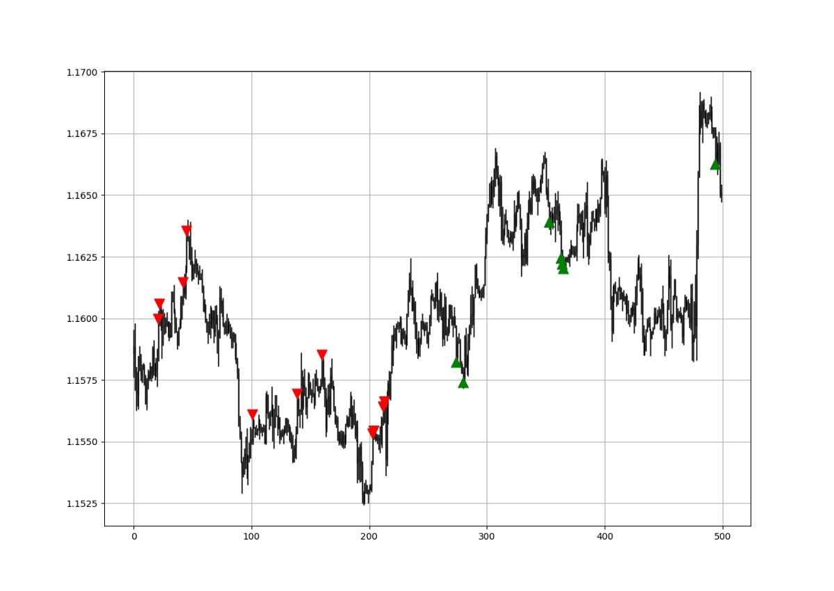
The exit conditions can be as follows. Note that it allows us to have multiple positions of the same kind to be open until the exit condition is satisfied.
# Buy Orders
for i in range(len(my_data)):

    try:

        if my_data[i, 7] == 1:

            for a in range(i + 1, i + 1000):

                if my_data[a, 3] >=  my_data[a, 4]:

                    if my_data[a, 9] == 0:

                        my_data[a, 9] = my_data[a, 3] - my_data[i, 3]
                        break

                    elif my_data[a, 9] != 0:

                        my_data[a, 9] = my_data[a, 9] + (my_data[a, 3] - my_data[i, 3])
                        break

                else:

                    continue

        else:

            continue

    except IndexError:

        pass

# Sell Orders
for i in range(len(my_data)):

    try:

        if my_data[i, 8] == -1:

            for a in range(i + 1, i + 1000):

                if my_data[a, 3] <=  my_data[a, 4]:

                    if my_data[a, 10] == 0:

                        my_data[a, 10] = my_data[i, 3] - my_data[a, 3]
                        break

                    elif my_data[a, 10] != 0:

                        my_data[a, 10] = my_data[a, 10] + (my_data[i, 3] - my_data[a, 3])
                        break

                else:

                    continue

        else:

            continue

    except IndexError:

        pass
The hit ratio on the strategy was 78.00% with a risk-reward ratio of 0.47. This can be considered as a strategy with a high potential, however, remember, that we did not account for transaction costs. Also, no optimization has been done as the above tests the theoretical strategy presented in the book. I have noticed that by tweaking the exit moving average, we get more stable and better results.
Conclusion
Remember to always do your back-tests. You should always believe that other people are wrong. My indicators and style of trading may work for me but maybe not for you.
I am a firm believer of not spoon-feeding. I have learnt by doing and not by copying. You should get the idea, the function, the intuition, the conditions of the strategy, and then elaborate (an even better) one yourself so that you back-test and improve it before deciding to take it live or to eliminate it. My choice of not providing specific Back-testing results should lead the reader to explore more herself the strategy and work on it more.
To sum up, are the strategies I provide realistic? Yes, but only by optimizing the environment (robust algorithm, low costs, honest broker, proper risk management, and order management). Are the strategies provided only for the sole use of trading? No, it is to stimulate brainstorming and getting more trading ideas as we are all sick of hearing about an oversold RSI as a reason to go short or a resistance being surpassed as a reason to go long. I am trying to introduce a new field called Objective Technical Analysis where we use hard data to judge our techniques rather than rely on outdated classical methods.
Keep reading with a 7-day free trial
Subscribe to All About Trading! to keep reading this post and get 7 days of free access to the full post archives.