Trading is a combination of four things, research, implementation, risk management, and post-trade evaluation. The bulk of what we spend our time doing is the first two, meaning that we spend the vast majority of the time searching for a profitable strategy and implementing it (i.e. trading).
However, we forget that the pillar of trading is not losing money. It is even more important than gaining money because it is fine to spend time trading and still have the same capital or slightly less than to spend time trading and find yourself wiped out. In this article, we will discuss the third pillar as a way of enhancing returns and capital protection. Every trading strategy must be accompanied by its own personalized risk management protocol. One such protocol (or indicator) is the famous average true range.
The Concept of Volatility
To understand the average true range, we must first understand the concept of volatility. It is a key concept in finance, whoever masters it holds a tremendous edge in the markets.
Unfortunately, we cannot always measure and predict it with accuracy. Even though the concept is more important in options trading, we need it pretty much everywhere else. Traders cannot trade without volatility nor manage their positions and risk. Quantitative analysts and risk managers require volatility to be able to do their work. Before we discuss the different types of volatility, why not look at a graph that sums up the concept? Check out the below image to get you started.
You can code the above in Python yourself using the following snippet:
# Importing the necessary libraries
import numpy as np
import matplotlib.pyplot as plt
# Creating high volatility noise
hv_noise = np.random.normal(0, 1, 250)# Creating low volatility noise
lv_noise = np.random.normal(0, 0.1, 250)# Plotting
plt.plot(hv_noise, color = 'red', linewidth = 1.5, label = 'High Volatility')
plt.plot(lv_noise, color = 'green', linewidth = 1.5, label = 'Low Volatility')plt.axhline(y = 0, color = 'black', linewidth = 1)
plt.grid()
plt.legend()The different types of volatility around us can be summed up in the following:
Historical volatility: It is the realized volatility over a certain period of time. Even though it is backward looking, historical volatility is used more often than not as an expectation of future volatility. One example of a historical measure is the standard deviation, which we will see later. Another example is the Average True Range, the protagonist of this article.
Implied volatility: In its simplest definition, implied volatility is the measure that when inputted into the Black-Scholes equation, gives out the option’s market price. It is considered as the expected future actual volatility by market participants. It has one time scale, the option’s expiration.
Forward volatility: It is the volatility over a specific period in the future.
Actual volatility: It is the amount of volatility at any given time. Also known as local volatility, this measure is hard to calculate and has no time scale.
The most basic type of volatility is our old friend “the Standard Deviation”. It is one of the pillars of descriptive statistics and an important element in some technical indicators (such as the Bollinger Bands). But first let us define what variance is before we find Standard Deviation:
Variance is the squared deviations from the mean (a dispersion measure), we take the square deviations so as to force the distance from the mean to be non-negative, finally we take the square root to make the measure have the same units as the mean, in a way we are comparing apples to apples (mean to standard deviation standard deviation). Variance is calculated through this formula:
Following our logic, standard deviation is therefore:
Therefore, if we want to understand the concept in layman’s terms, we can say that Standard Deviation is the average distance away from the mean that we expect to find when we analyze the different components of the time series.
Let us now keep the concept of being away from the mean in our heads and move away to the concept of the Average True Range.
Creating the Average True Range Indicator
In technical analysis, an indicator called the Average True Range -ATR- can be used as a gauge for historical volatility. Although it is considered as a lagging indicator, it gives some insights as to where volatility is now and where has it been last period (day, week, month, etc.).
But first, we should understand how the True Range is calculated (the ATR is just the average of that calculation). Consider an OHLC data composed of an timely arrange Open, High, Low, and Close prices. For each time period (bar), the true range is simply the greatest of the three price differences:
High — Low
High — Previous close
Previous close — Low
Once we have got the maximum out of the above three, we simply take a smoothed average of n periods of the true ranges to get the Average True Range. Generally, since in periods of panic and price depreciation we see volatility go up, the ATR will most likely trend higher during these periods, similarly in times of steady uptrends or downtrends, the ATR will tend to go lower. One should always remember that this indicator is very lagging and therefore has to be used with extreme caution.
Since it has been created by Wilder Wiles, also the creator of the Relative Strength Index, it uses Wilder’s own type of moving average, the smoothed kind. To simplify things, the smoothed moving average can be found through a simple transformation of the exponential moving average.
The above formula means that a 100 smoothed moving average is the same thing as (100 x 2) -1 = 199 exponential moving average. While we are on that, we can code the exponential moving average using this function:
def ma(data, lookback, close, where):

    data = adder(data, 1)

    for i in range(len(data)):

            try:

                data[i, where] = (data[i - lookback + 1:i + 1, close].mean())

            except IndexError:

                pass

    data = jump(data, lookback)

    return data
def ema(data, alpha, lookback, what, where):
alpha = alpha / (lookback + 1.0)
beta = 1 - alpha
data = ma(data, lookback, what, where)data[lookback + 1, where] = (data[lookback + 1, what] * alpha) + (data[lookback, where] * beta)for i in range(lookback + 2, len(data)):
try:
data[i, where] = (data[i, what] * alpha) + (data[i - 1, where] * beta)
except IndexError:
pass
return dataBelow is the function code that calculates a form of the ATR.
def atr(data, lookback, high, low, close, where):

    data = adder(data, 1)

    for i in range(len(data)):

        try:

            data[i, where] = max(data[i, high] - data[i, low], abs(data[i, high] - data[i - 1, close]), abs(data[i, low]  - data[i - 1, close]))

        except ValueError:

            pass

    data[0, where] = 0

    data = ema(data, 2, (lookback * 2) - 1, where, where + 1)
data = deleter(data, where, 1)
data = jump(data, lookback)
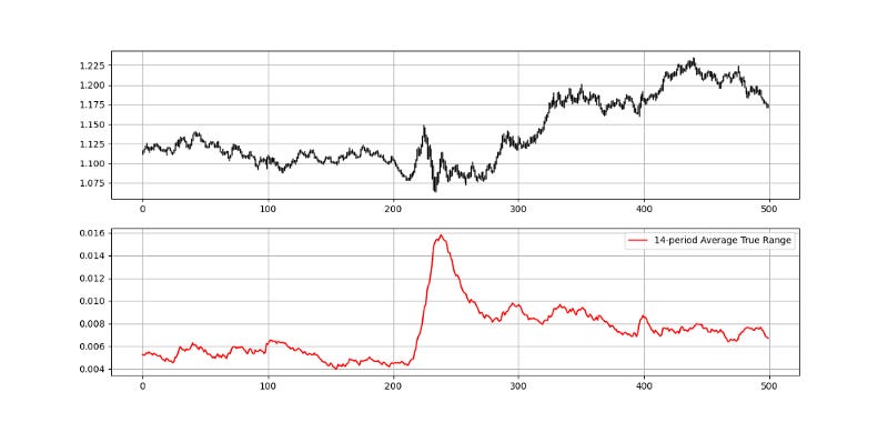
return dataLet us try applying the code on OHLC data and see the plot of a 14-period average true range:
Using the Average True Range in Risk Management
When I say I use ATR-based risk management system (Average True Range), it means that the algorithm will do the following steps with regards to the position it takes.
A long (Buy) position:
The algorithm initiates a buy order after a signal has been generated following a certain strategy.
Then, the algorithm will monitor the ticks and whenever the high equals a certain constant multiplied by ATR value at the time of the trade inception, an exit (at profit) order is initiated. Simultaneously, if a low equals a certain constant multiplied by ATR value at the time of the trade inception is seen, an exit (at loss) is initiated. The exit encountered first is naturally the taken event.
A short (Sell) position:
The algorithm initiates a short sell order after a signal has been generated following a certain strategy.
Then, the algorithm will monitor the ticks and whenever the low equals a certain constant multiplied by ATR value at the time of the trade inception, an exit (at profit) order is initiated. Simultaneously, if a high equals a certain constant multiplied by ATR value at the time of the trade inception is seen, an exit (at loss) is initiated. The exit encountered first is naturally the taken event.
The plot above shows the average true range. Take a look at the latest value on the ATR. It is around 0.0006 (6 pips). If we initiate a buy order following a simple 2.00 risk-reward ratio (risking half of what we expect to gain), we can place an order this way:
Buy at current market price.
Take profit at current market price + (2 x 6 pips).
Stop the position at current market price — (1 x 6 pips).
Conclusion
Remember to always do your back-tests. You should always believe that other people are wrong. My indicators and style of trading may work for me but maybe not for you.
I am a firm believer of not spoon-feeding. I have learnt by doing and not by copying. You should get the idea, the function, the intuition, the conditions of the strategy, and then elaborate (an even better) one yourself so that you back-test and improve it before deciding to take it live or to eliminate it. My choice of not providing specific Back-testing results should lead the reader to explore more herself the strategy and work on it more.
To sum up, are the strategies I provide realistic? Yes, but only by optimizing the environment (robust algorithm, low costs, honest broker, proper risk management, and order management). Are the strategies provided only for the sole use of trading? No, it is to stimulate brainstorming and getting more trading ideas as we are all sick of hearing about an oversold RSI as a reason to go short or a resistance being surpassed as a reason to go long. I am trying to introduce a new field called Objective Technical Analysis where we use hard data to judge our techniques rather than rely on outdated classical methods.
One Last Word
I have recently started an NFT collection that aims to support different humanitarian and medical causes. The Society of Light is a set of limited collectibles which will help make the world slightly better as each sale will see a percentage of it sent directly to the charity attributed to the avatar. As I always say, nothing better than a bullet list to outline the benefits of buying these NFT’s:
High-potential gain: By concentrating the remaining sales proceedings on marketing and promoting The Society of Light, I am aiming to maximize their value as much as possible in the secondary market. Remember that trading in the secondary market also means that a portion of royalties will be donated to the same charity.
Art collection and portfolio diversification: Having a collection of avatars that symbolize good deeds is truly satisfying. Investing does not need to only have selfish needs even though there is nothing wrong with investing to make money. But what about investing to make money, help others, and collect art?
Donating to your preferred cause(s): This is a flexible way of allocating different funds to your charities.
A free copy of my book in PDF: Any buyer of any NFT will receive a free copy of my latest book shown in the link of the article.


